Power analysis for cross-sectional and longitudinal study designs

Naiji LU, Yu HAN, Tian CHEN, Douglas D. GUNZLER, Yinglin XIA, Julia Y. LIN, Xin M. TU,5*

?Biostatistics in psychiatry (16)?

Power analysis for cross-sectional and longitudinal study designs

Naiji LU1,2, Yu HAN1, Tian CHEN1, Douglas D. GUNZLER3, Yinglin XIA1,2, Julia Y. LIN4, Xin M. TU1,2,5*

1. Introduction

Power and sample size estimation constitutes an important component of designing and planning modern scientific studies. It provides information for assessing the feasibility of a study to detect treatment effects and for estimating the resources needed to conduct the project. This tutorial discusses the basic concepts of power analysis and the major differences between hypothesis testing and power analyses. We also discuss the advantages of longitudinal studies compared to cross-sectional studies and the statistical issues involved when designing such studies. These points are illustrated with a series of examples.

2. Hypothesis testing, sampling distributions and power

In most studies we do not have access to the entire population of interest because of the prohibitively high cost of identifying and assessing every subject in the population. To overcome this limitation we make inferences about features of interest in our population, such as average income or prevalence of alcohol abuse, based on a relatively small group of subjects, or a sample, from the study population. Such a feature of interest is called a parameter, which is often unobserved unless every subject in the population is assessed. However, we can observe an estimate of the parameter in the study sample; this quantity is called a statistic. Since the value of the statistic is based on a particular sample, it is generally different from the value of the parameter in the population as a whole.Statistical analysis uses information from the statistic to make inferences about the parameter.

For example, suppose we are interested in the prevalence of major depression in a city with one million people.The parameter π is the prevalence of major depression.By taking a random sample of the population, we can compute the statistic p, the proportion of subjects with major depression in the sample. The sample size, n, is usually quite small relative to the population size. The statistic p will most likely not be equal to the parameter π because p is based on the sample and thus will vary from sample to sample. The spread by which p deviates from π with repeated sampling, is called sampling error.As long as n is less than 1,000,000, there will always be some sampling error. Although we do not know exactly how large this error is for a particular sample, we can characterize the sampling errors of repeated samples through the sampling distribution of the statistic. In the major depression prevalence example above, the behavior of the estimate p can be characterized by the binomial distribution. The distribution is more likely to have a peak around the true value of the parameter as the sample size n gets larger, that is, the larger the sample size n, the smaller the sampling error.

If we want to have more accurate estimates of a parameter, we need to have an n large enough so that sampling error will be reasonably small. If n is too small,the estimate will tend to be too imprecise to be of much use. On the other hand, there is also a point of diminishing returns, beyond which increasing n provides little added precision.

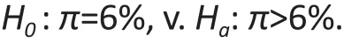
Power analysis helps to find the sample size that achieves the desired level of precision. Although research questions vary, data and power analyses all center on testing statistical hypotheses. A statistical hypothesis expresses our belief about the parameter of interest in a form that can be examined through statistical analysis. For example, in the major depression example, if we believe that the prevalence of major depression in this particular population exceeds the national average of 6%, we can express this belief in the form of a null hypothesis (H0) and an alternative hypothesis (Ha):Statistical analysis estimates how likely it is to observe the data we obtained from the sample if the null hypothesis H0was true. If it is very unlikely for us to observe the data we have if H0was true, then we reject the H0.

Thus, there are four possible decision outcomes of statistical hypothesis testing as summarized in the table below.

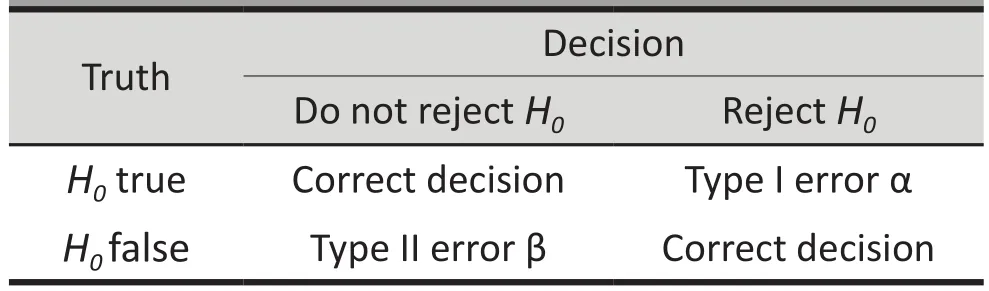
Decision outcomes of hypothesis testing

There are two types of errors associated with the decision to reject and not reject the null hypothesis H0.The type I error α is committed if we reject the H0when the H0is true; the type II error β occurs when we fail to reject the H0when the H0is false. In general, α (the risk of committing a type I error) is set at 0.05. The statistical power for detecting a certain departure from the H0(computed as 1–β), is typically set at 0.80 or higher; thus β(the risk of committing a type II error) is set at 0.20 or less.

3. Difference between hypothesis testing and power analysis

3.1 Hypothesis testing

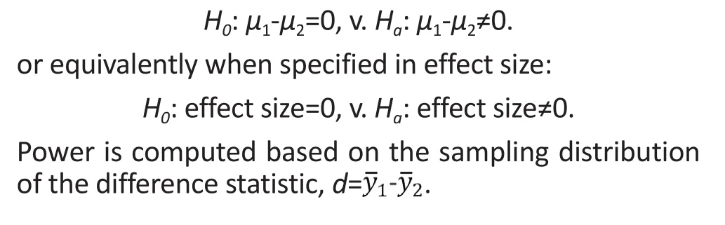
In most hypothesis testing, we are interested in ascertaining whether there is evidence against the H0based on the level of statistical significance. Consider a study comparing two groups with respect to some outcome of interest y. If μ1and μ2denote the averages of y for groups 1 and 2 in the population, one could make the following hypotheses:

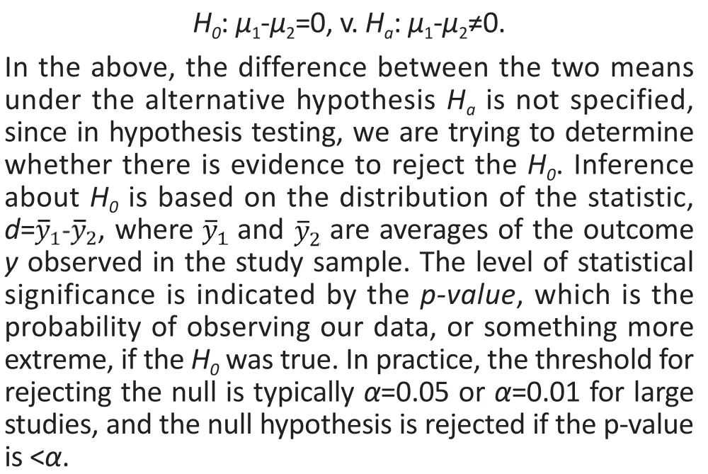
Note that no direction of effect is specified in the two-sided alternative Haabove; that is, we do not specify whether the average for group 1 is greater or smaller than the average for group 2. If we hypothesize the direction of effect a one-sided Hamay be used. For example:

3.2 Power analysis

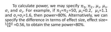
Unlike hypothesis testing, both the null H0and alternative Hahypotheses must be fully considered when performing power analysis. The usual purposes of conducting power analyses are (a) to estimate the minimum sample size needed in a proposed study to detect an effect of a certain magnitude at a given level of statistical power,or (b) to determine the level of statistical power in a completed study for detecting an effect of a certain magnitude given the sample size in the study. In the example above, to estimate the minimum sample size needed or to compute the statistical power, we must specify a value for δ=μ1-μ2, the difference between the two group averages, that we wish to detect under the Ha.

In power analysis, effects are often specified in terms of effect sizes, not in terms of the absolute magnitude of the hypothesized effect, because the magnitude of the effect depends on how the outcome is defined (i.e., what type of measures are employed) and does not account for the variability of such outcome measures in the study population. For example, if the outcome y is body weight, this could be alternatively measured in pounds or kilograms, the difference between two group averages could be reported either as 11 pounds or 5 kilograms. To remove dependence on the type of measure employed and account for variability of the outcomes in the study population,effect size – as standardized measure of the difference between groups – is often used to quantify hypothesized effect:

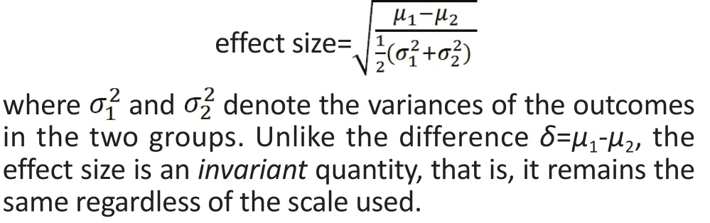
Note that effect sizes are different for different analytical models. For example, in regression analysis the effect size is commonly based on the change in R2, a measure for the amount of variability in the response (dependent) variable that is explained by the explanatory (independent) variables. Regardless of such differences, the effect size is a unitless quantity.

4. Examples of power analysis

4.1 Example 1

Consider again the hypothesis to test difference in average outcomes between two groups:

4.2 Example 2

Consider a linear regression model for a response(outcome) variable that is continuous with m explanatory(independent) variables in the model. The most common hypothesis is whether the explanatory variables jointly explain the variability in the response variable. Power is based on the sampling F-distribution of a statistic measuring the strength of the linear relationship between the response and explanatory variables and is a function of m, R2(effect size) and sample size n.

If m=5, we need a sample size of n=100 to detect an increase of 0.12 in R2with 80% power and α=0.05. Note that R is also called the multiple correlation coefficient or coefficient of multiple determination.

4.3 Example 3

Consider a logistic regression model for assessing risk factors of suicide. First, consider the case with only one risk factor such as major depression (predictor).The sample size is a function of the overall suicide rate π in the study population, odds ratio for the risk factor, and level of statistical power. The table below shows sample size estimates as a function of these parameters, with α=0.05 and power=80%. As shown in the table, if π=0.5,a sample size of n=272 is needed to detect an odds ratio of 2.0 for the risk variable (major depression) in the logistic model.

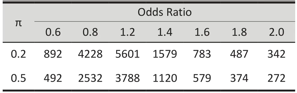
Sample sizes need to have an 80% power to detect different odds ratios at two different prevalence levels (π) of the target variable of interest

In many studies, we consider multiple risk factors or one risk factor controlling for other covariates. In this case, we first calculate the sample size needed for the risk variable of interest and then adjust it to account for the presence of other risk variables (covariates).

4.4 Example 4

Consider a drug-abuse study comparing parental conflict and parenting behavior of parents from families with a drug-abusing father (DA) to that of families with an alcohol-abusing father (AA). Each study participant is assessed at three time points. For such longitudinal studies, power is a function of within-subject correlation ρ, that is, the correlation between the repeated measurements within a participant. There are many data structures that can be used to assess this within-subject correlation; the details for doing this can be found in the paper by Jennrich and Schluchter.[1]

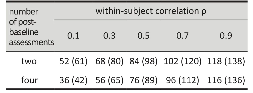
Required sample sizes for complete data (and 15%missing data) to detect differences in an outcome of interest between two groups (α=0.05; β=0.20) when the outcome is assessed repeatedly and there are different levels of within-subject correlation

As seen in the above table, the sample sizes required to detect the desired effect size increased as ρ approaches 1 and decreased as ρ approaches 0. Sample size also depends on the number of post-baseline assessments,with smaller sample sizes needed when there are more assessments. In the extreme case when ρ=0 (there is no relationship between the repeated assessment within a participant) or ρ=1 (repeated assessments within a participant yield identical data), the repeated outcomes become completely independent (as if they were collected from other individuals) or redundant (providing no additional information).

When ρ=1, all repeated assessments within a participant are identical to each other, and thus the additional assessments do not yield any new information. In comparison, when ρ≠1, longitudinal studies always provide more statistical power than their cross-sectional counterparts. Furthermore, the sample size required is smaller when ρ approaches 0, because repeated measurements are less similar to each other and provide additional information on the participants. To ensure reasonably small within-subject correlations, researchers should avoid scheduling post-baseline assessments too close to each other in time.

In practice, missing data is inevitable. Since most commercial statistical packages do not consider missing data, we need to perform adjustments to account for its effect on power. One way of doing this (shown in the table) is to inflate the estimated sample size. For example, if it is expected that 15% of the data will be missing at each follow-up visit and n is the estimated sample size needed under the assumption of complete data, we inflate the sample size n’=n/(1-15%). As seen in the table, missing data can have a sizable effect on the estimated sample sizes needed so it is important to have good estimates of the expected rate of missing data when estimating the required sample size for a proposed study. It is equally important to try to reduce the amount of missing data during the course of the study to improve statistical power of the results.

5. Software packages

Different statistical software packages can be used for power analysis. Although popular data analysis packages such as R[2]and SAS[3]may be used for power analysis, they are somewhat limited in their application,so it is often necessary to use more specialized software packages for power analysis. We used PASS 11[4]for all the examples in this paper. As noted earlier, most packages do not accommodate missing data for longitudinal study designs, so ad-hoc adjustments are necessary to account for missing data.

6. Discussion

We discussed power analysis for a range of statistical models. Although different statistical models require different methods and input parameters for power analysis, the goals of the analysis are the same: either(a) to determine the power to detect a certain effect size (and reject the null hypothesis) for a given sample size, or (b) to estimate the sample size needed to detect a certain effect size (and reject the null hypothesis) at a specified power. Power analysis for longitudinal studies is complex because within-subject correlation, number of repeated assessments, and level of missing data can all affect the estimations of the required sample sizes.

When conducting power analysis one needs to specify the desired effect size, that is, the minimum magnitude of the standardized difference between groups that would be considered relevant or important. There are two common approaches for determining the effect sizes used when conducting power analyses: use a ‘clinically significant’ difference; and use information from published studies or pilot data about the magnitude of the difference that is common or considered important.When using the second approach, one must be mindful of the sample sizes in prior studies because reported averages, standard deviations, and effect sizes can be quite variable, particularly for small studies. And the previous reports may focus on different population cohorts or use different study designs than those intended for the study of interest so it may not be appropriate to use the prior estimates in the proposed study. Further, given that studies with larger effect sizes are more likely to achieve statistical significance and,hence, more likely to be published, estimates from published studies may overestimate the true effect size.

Conflict of interest

The authors report no conflict of interest related to this manuscript.

Acknowledgments

This research is supported in part by the Clinical and Translational Science Collaborative of Cleveland,UL1TR000439, and of the University of Rochester,5-27607, from the National Institutes of Health.

1. Jennrich RI, Schluchter MD. Unbalanced repeated-measures models with structured covariance matrices. Biometrics 1986; 42: 805–820.

2. R Core Team. R: A Language and Environment for Statistical Computing. R Foundation for Statistical Computing: Vienna,Austria, 2012. ISBN 3-900051-07-0, URL http://www.R-project.org/. R Package ‘pwr’http://cran.r-project.org/web/packages/pwr/index.html

3. Castelloe JM. Sample Size Computations and Power Analysis with the SAS System. Proceedings of the Twenty-Fifth Annual SAS Users Group International Conference; [April 9-12,2000]; Indianapolis, Indiana, USA; Cary, NC: SAS Institute Inc.; 265-25.

4. Hintze J. PASS 11. NCSS, LLC. Kaysville, Utah, USA, 2011.

10.3969/j.issn.1002-0829.2013.04.009

1Department of Biostatistics, University of Rochester Medical Center, Rochester, NY, USA

2Veterans Integrated Service Network 2 Center of Excellence for Suicide Prevention, Canandaigua VA Medical Center, Canandaigua, NY, USA

3School of Medicine, Case Western Reserve University, Center for Health Care Research & Policy, MetroHealth Medical Center, Cleveland, OH, USA

4US Department of Veterans Affairs Cooperative Studies Program Coordinating Center, Palo Alto VA Health Care System, Palo Alto, CA, USA

5Department of Psychiatry, University of Rochester Medical Center, Rochester, NY, USA

*correspondence: xin_tu@urmc.rochester.edu

Naiji Lu received his PhD. from the Mathematics Department of the University of Rochester in 2007 after completing his thesis on Branching Process. He is currently a Research Assistant Professor in the Department of Biostatistics and Computational Biology at the University of Rochester Medical Center.Dr. Lu’s research interests include social network analysis, longitudinal data analysis, distribution-free models, robust statistics, causal effect models, and structural equation models as applied to large complex clinical trials in psychosocial research.