Heterogeneity of treatment effects

Naihua DUAN*, Yuanjia WANG

· Biostatistics in Psychiatry (7) ·

Heterogeneity of treatment effects

Naihua DUAN1,2*, Yuanjia WANG1,2

In many clinical studies it is important to examine whether or not the effect of the treatment varies across patient subgroups[1]. For example, does the effect of treatment for depression with a specific SSRI vary by gender? In other words, is there ‘heterogeneity of treatment effects’ (HTE)? This information is important for clinical decision-making; clinicians can target a specific treatment to patients who are expected to benefit most from the treatment and seek alternative treatments for patients who are expected to benefit least from the treatment.

A common mistake in studies that compare treatment effects across subgroups (HTE studies) is to assume that differences in the statistical significance(p-value) of the treatment effect in different subgroups indicates that the treatment effect in the subgroups is different. For example, in a medication trial for major depression investigators who find that the treatment effect is statistically significant among females but insignificant among males may incorrectly conclude that the treatment effect differs by gender and recommend the treatment be used for females but not for males.The problem with this conclusion is that statistical significance is determined not only by the treatment effect but also by the sample size and other study design factors.

Despite the different observed statistical significance in this hypothetical study, it is possible that a further examination of the data might reveal that the effect size for the medication treatment was essentially the same for males and females. As an example , assume that there is a 7.5 point mean difference in the change of the Hamilton Rating Scale for Depression (HAMD)during treatment for females on medication versus females on placebo but a 8.1 point mean difference for males on medication versus males on placebo (that is,the treatment effect is slightly greater for males than females). Let us also assume that the number of women participating in this hypothetical study is substantially larger than the number of men participating in the study because of the much higher prevalence of depression among females than among males. As a result of the substantial difference in gender-specific sample sizes, it is possible that the treatment effect of 7.5 points among females turns out to be statistically significant while the slightly larger treatment effect of 8.1 points among males turns out to be statistically insignificant. Therefore, the difference in the statistical significance between males and females might be the result of differences in the gender-specific sample sizes; it does not necessarily reflect a difference in the treatment effects.

The appropriate statistical method for studying the HTE is to test for the statistical interaction between treatment and the covariate of interest, such as patient’s gender. The need to examine statistical interactions was mentioned in previous columns in this series[2,3]. We provide a more detailed discussion of statistical interactions for continuous outcome measures below.

In our hypothetical example the statistical interaction between treatment and gender compares the treatment effect for females with the treatment effect for males. For a continuous outcome measures such as the HAMD, the statistical model can be formulated as a standard linear regression model,with the usual assumptions for the error distribution(normality and homoscedasticity):

where DH denotes the pre-post change in HAMD,TX denotes treatment assignment (TX=1 for active medication, TX=0 for placebo), FG denotes female gender (FG=1 for females, FG=0 for males), and TXFG is the interaction term:

The remaining terms in Model (1) are unobserved parameters to be estimated: b0 denotes the intercept term, b1 denotes the “main effect” for treatment(active medication compared to placebo), b2 denotes the “main effect” for gender (females compared to males), b3 denotes the interaction between treatment and gender (treatment effect among females compared to treatment effect among males), and e denotes the residual variation.

It is important to note that the presence of the interaction term in the model changes the usual interpretation of the other parameters. The “main effect” for treatment, b1, does not represent the overall effect of treatment in the full sample but, rather, the effect of treatment for males (when the FG covariate is 0). And the “main effect” for gender, b2, does not represent the overall effect for gender for the entire sample but, rather, the effect for gender in the placebo group (when TX=0). More specifically, the expected outcomes in Model (1) for patients with the various combinations of treatment and gender are given as follows in Table 1 (the residual variation term ‘e’ is dropped):

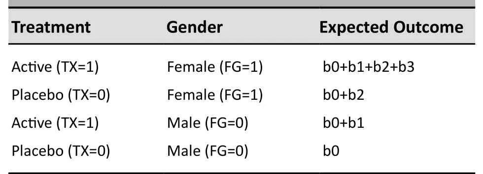
Table 1. The expected outcomes with various treatment and gender

Comparing the first two rows in the table above, it can be seen that the treatment effect (active medication vs. placebo) among females is given by

Similarly, comparing the third and fourth rows in the table above, it can be seen that the treatment effect among males is given by

Comparing Equations (3) and (4), it can be seen that the interaction between treatment and gender (treatment effect among females compared to treatment effect among males) is given by

The point estimate, confidence interval, and statistical significance for the interaction effect, b3, are provided directly by statistical software packages such as SAS and SPSS as part of the software’s standard analysis output.These values indicate the likelihood that the treatment effect is, in fact, different for men and women.

This analysis is also useful for assessing the treatment effect in each patient subgroup. As stated above and shown in equation (4), when the interaction term is in the model the b1 parameter estimates the treatment effect for the subgroup in which the gender covariate is null, which is the subgroup of males in this example. In this situation the point estimate,confidence interval and statistical significance of the‘main effect for gender’ provided by standard statistical software would indicate the treatment effect for the male subgroup.

Computation of the treatment effect for the subgroup in which the gender covariate is not null(females in this example) is more complicated. As shown in Equation (3), the treatment effect among females is given by b1 + b3. While it is straightforward to obtain the point estimate for the combination b1 + b3 (by summing the point estimates provided in the standard output), it is not straightforward to obtain information about the confidence interval and statistical significance for the combination b1 + b3. These parameters can be obtained using sophisticated software but it is generally easier to simply reverse the coding for the covariate for gender (making female=0 and male=1) and re-running the analysis:

Here, MG is the indicator variable for males: MG=1 for males and MG=0 for females. The analysis is then rerun with the terms MG and TXMG replacing FG and TXFG in Model (1):

With the alternative specification in Model (1’) instead of Model (1), the interaction effect remains unchanged– the coefficient for TXMG in Model (1’) is the same as the coefficient for TXFG in Model (1):

Therefore, either Model (1) or Model (1’) can be used to assess the interaction effect between treatment and gender. (Equation (8) can be shown by constructing a table for Model (1’) similar to the earlier table for Model (1).)

The parameter c1 in Model (1’) represents the treatment effect for females (the subgroup of patients with null value [MG=0] for the covariate MG). In other words, the parameter c1 in Model (1’) is related to the parameters in Model (1) as follows:

Therefore, with Model (1’), the standard analysis output for the ‘main effect of gender’ is the point estimate,confidence interval, and statistical significance for the treatment effect among female patients, represented by the parameter c1 in Model (1’).

1. Kravitz RL, Duan N, Braslow J. Evidence-based medicine,heterogeneity of treatment effects, and the trouble with averages. Milbank Q, 2004, 82(4): 661-687. Erratum in: Milbank Q, 2006, 84(4): 759-760.

2. Lin JY, Lu Y. Estimating treatment effects in observational studies.Shanghai Arch Psychiatry, 2011, 23(6): 380-382.

3. Liu X. Binary outcome variables and logistic regression models.Shanghai Arch Psychiatry, 2011, 23(5): 318-320.

10.3969/j.issn.1002-0829.2012.01.006

1Department of Biostatistics, Mailman School of Public Health, Columbia University, New York, USA

2Division of Biostatistics, Department of Psychiatry, Columbia University Medical Center, New York, USA

*Correspondence: naihua.duan@columbia.edu