Modelling of Nanoscale Friction using Network Simulation Method

F.Marín,F.Alhamaand J.A.Moreno

1 Introduction

The physical phenomenon of dry friction between sliding bodies is an important subject in mechanical engineering,to which many studies have been devoted[Blau(1986);Dowson(1998);Perry(2001);Blau(2001);Müser(2006)].In nanotribology,the frictional behaviour of a single-asperity contact should first be investigated to improve our understanding of friction in macroscopic systems.Once the atomicscale manifestations of friction at such a nanometre-sized single asperity have been clarified,macroscopic friction can be explained with the summation of the interactions of a large number of small individual contacts,which form the macroscopic roughness of the contact interface[H?lscher,Schirmeisen and Schwarz(2008)].

In recent decades,the field of nanotribology has become firmly established through the introduction of new experimental tools,which have made nanometric and atomic scales accessible to tribologists[Bhushan,Israelachvili and Landmann(1995);Carpick,Ogletree and Salmeron(1997);Urbakh,Klafter,Gourdon and Israelachvili(2004)].While surface force apparatus(SFA)is generally used with molecular thick liquid films sandwiched between atomically smooth surfaces,atomic force microscopy/friction force microscopy(AFM/FFM),a technique derived from scanning force microscopy(SFM),simulates a solid-solid interface with numerous asperities.These techniques are increasingly used for tribological studies of engineering surfaces at scales ranging from atomic and molecular to micro;such studies including surface roughness,adhesion,friction,scratching,wear,indentation,the detection of material transfer and boundary lubrication[Bhushan(2000);H?lscher,Schwarz and Wiesendanger(1996)].

However,theoretical understanding of the individual processes involved in friction force microscopy is still insufficient[H?lscher,Schwarz and Wiesendanger(1996)],and numerical simulations are crucial in this respect.Indeed,simulations have evolved since the first simple theoretical models of friction at atomic scale[Tomlinson(1929);Frenkel and Kontorova(1938);Alhama,Marín and Moreno(2011)]which were applied to the friction force microscope[Zhong and Toánek(1990);Tománek,Zhong and Thomas(1991);Gyalog,Bammerlin,?uthi,Meyer and Thomas(1995)]and which are able to explain essential features of atomic friction processes.Nowadays,theoretical simulations of AFM images for systems include movable substances like flakes or molecules on surfaces[Miura,Sasaki and Kamiya(2004);Verhoeven,Dienwiebel and Frenken(2004)].In this way,molecular-dynamics simulations provide valuable insight into atomic processes and interactions,but still need much computer time to provide quantitative results[H?lscher,Schwarz and Wiesendanger(1996)].

The aim of this work was to design a reliable and efficient model for nanoscale friction,following the rules of network simulation[González-Fernández(2001)],which can be simulated in commercial circuit analysis software such as PSpice[Microsim Corporation(1994);Nagel(1977)].The model,which provides both transient and steady state solutions,is based on the formal equivalence between the differential equations of the mathematical and network models,going beyond the scope of classical electrical analogy of many books[Kreith(2000);Mills(1998)]which mainly deal with linear problems.The network method is a numerical tool whose efficiency has been demonstrated in many science and engineering problems,such as heat transfer,electrochemistry, fluid flow and solute transport,inverse problems,etc[González-Fernández,Alhama and López-Sánchez(1998);Horno,González-Fernández and Hayas(1995);Soto,Alhama and González-Fernández(2007);Zueco and Alhama(2006)].Once the equivalence between electric and mechanical variables has been chosen,linear terms of the PDE are easily implemented by linear electrical devices such as resistors,capacitors and coils,while non-linear and coupled terms are implemented using auxiliary circuits or controlled current and voltage sources.The last are a special kind of source whose output can be defined(by software)as a function of the dependent or independent variables defined in any node or any electrical component of the model.In addition,boundary and initial conditions–linear or not–are also immediately implemented by suitable electric components.Once the network model has been designed,it is run with no need for other mathematical manipulations since the simulation code does this.The well-tried and powerful software for circuit simulation PSpice,requires relatively short computing times thanks to the continuous adjusting of the internal time step required for the convergence.In addition,the solution simultaneously provides all the variables of interest:displacements and velocities.

Compared with a wide variety of complex schemes,our network model provides a simple scheme to simulate the different microscopes used to study the phenomenon of friction on different sample surfaces,at nanometre and atomic scales,at the same time reducing the computational time needed.Despite of its simplicity,the network model is able to integrate a multiplicity of parameters,which either improve the accuracy of the simulation or integrate additional parameters.

2 The governing equations

The physical scheme of the FFM,AFM or SFM tip on a sample surface model,Fig.1,assumes one rigid sliding body connected by three springs(one for each spatial direction)to the mobile microscope support.Each spring reflects the elastic interaction between the two surfaces during the contact[H?lscher,Schwarz and Wiesendanger(1996);Sasaki,Kobayashi and Tsukada(1996)].The sliding body involves inertial effect and the interaction with the sample surface.

The hypotheses currently assumed in FFM,AFM and SFM models are:(i)the microscope support is rigid and moves at a constant velocity,vM,(ii)the cantilever and the tip show elastic behaviour,and(iii)interactional force between the tip and the sample surface is a function of the relative distances between the tip and the atoms forming the sample surface.

Several forces act on the tip in x-direction:inertial force represented by ‘m·(d2xt/dt2)’,where xtis the absolute displacement of the tip of mass m;elastic force from the spring,represented by the term ‘kx·(xM-xt)’;and damping force represented by the term ‘cx·(dxt/dt)’.The coefficients of these forces are constants.Similar forces act in the other directions.In addition,the interaction force between the tip and the sample surface is implemented from a surface potential[H?lscher,Schwarz and Wiesendanger(1996);Sasaki,Kobayashi and Tsukada(1996);H?lscher,Schwarz,Zw?rner and Wiesendanger(1998)].Thus,the surface potential for NaF with an FFM tip,as used by H?lscher et al.[H?lscher,Schwarz and Wiesendanger(1996)]is:

Figure 1:Model of AFM,FFM and SFM tip.

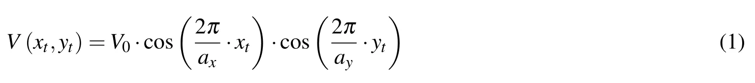
where the potential amplitude,V0,is 1 eV,while axand ay,the double of the lattice constant,are 4.62 ? for both parameters.The same surface potential formula is used by H?lscher et al.[H?lscher,Schwarz and Wiesendanger(1997)]for MoS2with SFM tip,where V0is equal to 1 eV and axand ayare equal to 3.16 ? and 5.48,respectively.H?lscher et al.[H?lscher,Schwarz,Zw?rner and Wiesendanger(1998)]use a slight modification of Eq.1 to study HOPG with a SFM tip:

where V0is 0.5 eV and the lattice constant,a,is 2.46 ?.

Sasaki et al.[Sasaki,Kobayashi and Tsukada(1996)]used the Lennard-Jones potential to study the graphite with an AFM tip:

昆明冶金研究院通過對霧化噴嘴的改進，在溫度1 800℃，霧化壓力2.0MPa條件下，采用氮氣霧化技術(shù)制備316 L不銹鋼金屬粉末，并與德國EOS公司粉體形貌進行對比，微觀結(jié)構(gòu)情況見圖3。

where the strength of the potential,ε,is 0.87381·10?2eV,and the value of the distance between the tip and the surface atom at which the potential is zero,σ,is 2.4945 ?.The distance between the tip and the i-th atom of the surface,r0i,is calculated from the i-th atom position inside the lattice,which is defined by its constant,2.46 ?,and the nearest distance between 2 carbon atoms,1.42 ?.H?lscher et al.used the same potential with the same sample surface and microscope[H?lscher,Allers,Schwarz,Schwarz and Wiesendanger(2000)],but σ is equal to 3.4 ?.The surface potential for xenon with an AFM tip used by H?lscher et al.[?lscher,Allers,Schwarz,Schwarz and Wiesendanger(2001)]is the same as that used in graphite.The value of σ is equal to 3.3 ?.

As a result of the balance of the forces on the tip,Fig.1,the following equations can be written:

The movement of the microscope support is a set of trips in the x-direction.For each of these trips,the initial condition of tip displacement in the x-direction is null,and in the z-direction is null except for the AFM tip on graphite and xenon sample.In the y-direction,the initial condition for this displacement is the same as for the microscope support.The initial condition of tip velocity is null for each direction.

3 The network model and the PS pice code

The design of a reliable network model requires a formal equivalence between the equations of the model and those of the process,including the initial conditions.Since Eq.4,the basic network model is related to this equation,to which initial conditions must be added.Basic rules for designing the model can be found in González-Fernández[González-Fernández(2001)].The first step is to choose the equivalence between mechanical and electric variables(different choices give rise to different networks).For the problem under consideration,the following equivalence is established:xt(tip displacement in the x-direction)≡q(electric charge in the network),ordxt/dt(tip velocity in the x-direction)≡dq/dt=i(electric current at the network).In the other directions,similar equivalences are applied.

Now,each term of the Eq.4 is considered as a voltage in an electric component whose constitutive equation is defined by the mathematical expression of such a term.Hence,the equation itself can be considered as a voltage balance(second Kirchhoff’s law)of a network that contains as many electrical components connected in series as there are terms in the equation.The linear term of Eq.4‘(d2xt/dt2)’is associated to a coil(inductance)since the constitutive equation of this component is VL=L(di/dt)=L(d2q/dt2),with L=1H.The same electrical ele-ment is used for the other two directions.The non-linear terms cannot be implemented directly,and require the use of controlled current(or voltage)sources or auxiliary circuits.The first are devices whose output is defined by software as an arbitrary,continuous mathematical function of the dependent variables:voltages at any node of the network or the current in any component.This capability,which is beyond the scope of the classical electrical analogy that appears in most text books,makes the network method an interesting and efficient tool in the field of numerical computation.

To implement the term ‘xt’,the value of this variable must be determined by integrating the current in the network model,dxt/dt.To this end,an auxiliary circuit is implemented,Fig.2(b),in the models of FFM on the NaF sample and SFM on the MoS2sample;Fig.3(c)in the model of AFM on a graphite sample;and Fig.4(c)in the model of AFM on xenon sample.The terms ytand ztare implemented in similar network models.F1xis the controlled current source whose output is the current,dxt/dt,that crosses the voltage generator(used as an ammeter),Vx.The voltage of this generator is zero so as not to disturb the network model of Eq.4.The current of F1xis integrated using a capacitor with Cx1=Cy1=Cx=1F;in this way,the voltage through this capacitor,VCx1=VCy1=VCx=C?1x∫(dxt/dt)dt,is simply the variable xt(a resistor of very high value,RINF,is needed for electrical continuity).

The initial conditions related to displacements,xM-xt=yM-yt=zM-zt=0,and velocities,dxt/dt=dyt/dt=dzt/dt=0,are introduced in the specifications of the initial conditions of the capacitors(initial voltage value)and of the coils(initial current value),respectively.The whole network model is now run in a Duo Core,using the code PSpice[Microsim Corporation(1994);Nagel(1977)]and very few rules are required since the model contains very few electrical devices.

Figure 2:Network model,in x and y directions,of FFM on NaF,SFM on MoS2 and SFM on HOPG.a)and d)Main circuits,b)and e)auxiliary circuits to obtain xtand yt,and c)auxiliary circuit to obtain the time.

Figure 3:Network model,in x direction,of AFM on graphite.a)Main circuit,b)auxiliary circuit to obtain the force from Lennard-Jones potential,c)auxiliary circuit to obtain xt,d)auxiliary circuit to obtain the time,and e)auxiliary circuit to obtain the square of the distance between the AFM tip and the carbon atom.

Figure 4:Network model,in x direction,of a AFM on xenon.a)Main circuit,b)auxiliary circuit to obtain the force from Lennard-Jones potential,c)auxiliary circuit to obtain xt,d)auxiliary circuit to obtain the time,and e)auxiliary circuit to obtain the square of the distance between the AFM tip and the xenon atom.

4 Applications

The Network Simulation Method has been applied to sample surfaces and tips for which data are available:FFM tip on NaF[H?lscher,Schwarz and Wiesendanger(1996)],AFM tip on Xe[?lscher,Allers,Schwarz,Schwarz and Wiesendanger(2001)],SFM tip on MoS2[H?lscher,Schwarz and Wiesendanger(1997)],SFM tip on HOPG[H?lscher,Schwarz,Zw?rner and Wiesendanger(1998)],and AFM tip on graphite[H?lscher,Allers,Schwarz,Schwarz and Wiesendanger(2000)].The first two samples have the same cubic crystal net and the others have a hexagonal crystal net,which tests the potential of the network model.

The characteristics of the tip,the test conditions and the sample size for the different tests are:

?the FFM tip on NaF sample is characterized by mx=my=10?8kg,cx=cy=10?3N·s/m and kx=ky=10 N/m.The microscope support moves with a constant velocity of 400 ?/s,and the results are depicted with a scan range of 20x20 ? and scan angle of 0°[H?lscher,Schwarz and Wiesendanger(1996)].The proposed model solves the Eq.4 using the potential defined in Eq.1.

?theAFMtiponXeis characterizedbycx=cy=0N·s/m,andkx=ky=kz=40N/m.The results are depicted with a scan range of 36x36 ? and scan angle of 15°[?lscher,Allers,Schwarz,Schwarz and Wiesendanger(2001)].Moreover,to obtain similar results to those obtained by the above authors,the following parameters were assumed:mx=my=10?6kg,a constant velocity of 10 ?/s for the microscope support,and a vertical displacement of-6 ? for the tip,parameters not mentioned by H?lscher et al.[?lscher,Allers,Schwarz,Schwarz and Wiesendanger(2001)].

?the SFM tip on MoS2sample is characterized by mx=my=10?8kg,cx=cy=10?3N·s/m and kx=ky=10 N/m.The microscope support moves with a constant velocity of 400 ?/s,and the results are depicted with a scan range of 25x25? and scan angle of0o[H?lscher,Schwarz and Wiesendanger(1997)].

?the SFM tip on HOPG sample is characterized by mx=my=10?8kg,cx=cy=10?3N·s/mandkx=ky=25N/m.The microscope support moves with constant velocity of 400 ?/s,and the results are depicted with a scan range of 20x20 ? and scan angle of 7o.The surface of the sample is composed of 271 hexagons with a carbon atom in each vertex(600 altogether);and it is assumed that the sample surface has a very high stiffness[H?lscher,Schwarz,Zw?rner and Wiesendanger(1998)].

?the AFM tip on graphite is characterized by cx=cy=0N·s/m,kx=ky=0.25-2.5 N/m,kz=0.25N/m,and a vertical displacement of-6? for the tip.The results are depicted with a scan range of 9.8x8.5 ? and scan angle of 15o[Sasaki,Kobayashi and Tsukada(1996)].Besides,mx=my=10?6kg and a constant velocity of 10 ?/s for the microscope support,parameters not mentioned by Sasaki et al.[Sasaki,Kobayashi and Tsukada(1996)],were assumed to obtain results similar to theirs.

Eq.4 is solved in each test for the potential functions defined in the following equations:

?Eq.1 in the FFM tip on NaF and in the SFM tip on MoS2sample models

?Eq.2 in the SFM tip on HOPG sample model

?Eq.3 in the AFM tip on Xe and graphite samples models

In the last case,for Xe and graphite samples,only short computational times are necessary for the software to find the right values of the parameters not supplied by H?lscher et al.[?lscher,Allers,Schwarz,Schwarz and Wiesendanger(2001)]and Sasaki et al.[Sasaki,Kobayashi and Tsukada(1996)],respectively.

Fig.5(b)shows the components of the tip elastic force,Fxand Fy,in each position on the NaF sample surface,whose crystal net is shown in Fig.5(a).The correspondence between both depicted images enables us to use this software as a tool to interpret those images from the microscope.Thus,this software is able to manage different theoretical crystal nets,even with crystallographic defects,providing the corresponding theoretical elastic forces,which can be compared with those from the microscope.The results of the simulation agree with those obtained by H?lscher et al.[H?lscher,Schwarz and Wiesendanger(1996)].

Fig.6(b)shows the x-direction component of the tip elastic force,Fx,in each position on the Xe sample surface,whose crystal net is shown in Fig.6(a).As mentioned for Fig.5(b),the results agree with those obtained by H?lscher et al.[?lscher,Allers,Schwarz,Schwarz and Wiesendanger(2001)].

Fig.7(b)shows the components of the tip elastic force,Fxand Fy,in each position on the MoS2sample surface,whose crystal net is shown in Fig.7(a).The results of the simulation agree with those obtained by H?lscher et al.[H?lscher,Schwarz and Wiesendanger(1997)].

Figure 5:a)Position of the atoms in the NaF crystal net b)Elastic force in the tip:Fxin the left hand side and Fyin the right hand side.

Figure 6:a)Position of the atoms in the xenon crystal net b)Elastic force in the tip,Fx.

Figure 7:a)Position of the atoms in the MoS2crystal net b)Elastic force in the tip:Fxin the left hand side and Fyin the right hand side.

Figure 8:a)Position of the atoms in the HOPG crystal net b)Elastic force in the tip:Fxin the left hand side and Fyin the right hand side.

Figure 9:a)Position of the atoms in the HOPG crystal net b)Elastic force in the tip,Fx.

Fig.8(b)shows the components of the tip elastic force,Fx and Fy,in each position on the HOPG sample surface,whose crystal net is shown in Fig.8(a).The results of the simulation agree with those obtained by H?lscher et al.[H?lscher,Schwarz,Zw?rner and Wiesendanger(1998)].Besides,Fig.9(b)shows the x-direction component of the tip elastic force,Fx,in each position on the graphite sample surface,whose crystal net is shown in Fig.9(a).In this case,a 3D graph is used to show the details better,to be more precise the stick–slip mechanism.The lines of the graph are traced at different y-coordinates,separated by a fixed step.When one of these lines crosses the sample surface at a critical position,the instabilities appear,Fig.9(b).These critical positions have a relation with the minimal threshold of the distance between the tip and the atom on the surface.The results of the simulation agree with those obtained by Sasaki et al.[Sasaki,Kobayashi and Tsukada(1996)].

5 Conclusions

A numerical model based on the network method has been designed to simulate several types of microscope and sample surfaces with different crystal nets.The results were successfully compared with those of different authors obtained with different methodologies.The software is flexible enough to implement the different values of the main parameters with no important changes,and allows different types of graph to be used.Thus,this software is able to manage different theoretical crystal nets,even with crystallographic defects,providing the corresponding theoretical elastic forces that can be compared with those obtained by microscope.Furthermore,the short computational time necessary means that the software can be used to determine the values of the microscope parameters from experimental images of certain materials,whose data are not available.The calculated parameters allow other sample materials to be simulated.The final potential use of this software is to test the effect of microscope parameters on the quality of the image assisting to the use of the microscope.

Alhama,F.;Marín,F.;Moreno,J.A.(2011):An efficient and reliable model to simulate microscopic mechanical friction in the Frenkel-Kontorova-Tomlinson model.Computer Physics Communications,vol.182,pp.2314-2325

Bhushan,B.(2000):Handbook of Modern Tribology.CRC Press:London,pp.717.

Bhushan,B.;Israelachvili,J.N.;Landmann,U.(1995):Nanotribology:friction,wear and lubrication at the atomic scale.Nature,vol.374,pp.607-616.

Blau,P.J.(1986):Friction Science and Technology.Marcel Dekker:New York,pp.285.

Blau,P.J.(2001):The significance and use of the friction coefficient.Tribology International,vol.34,pp.585-591.

Carpick,R.W.;Ogletree,D.F.;Salmeron,M.(1997):Lateral stiffness:a new nanomechanical measurement for the determination of shear strengths with friction force microscopy.Applied Physics Letters,vol.70,pp.1548–1550.

Dowson,D.(1998):History of Tribology.Professional Engineering Publishers:London,pp.43.

Frenkel,F.C;Kontorova,T.(1938):Zh.Eksp.Teor.Fiz.,vol.8,pp.1340.

González-Fernández,C.F.(2001):Heat transfer and the Network Simulation Method.J.Horno(Ed.):Research Signpost,Trivandrum,pp.30.

González-Fernández,C.F.;Alhama,F.;López-Sánchez,J.F.(1998):Application of the network method to heat conduction processes with polynomial and potential-exponentially varying termal properties.Numerical Heat Transfer.Part A-Applications,vol.33,no.5,pp.549-559.

Gyalog,T.;Bammerlin,M.;L?uthi,R.;Meyer,E.;Thomas,H.(1995):Mechanism of atomic friction.Europhysics Letters 1995,vol.31,pp.269-274

H?lscher,H.;Allers,W;Schwarz,U.D.;Schwarz,A.;Wiesendanger,R.(2001):Simulation of NC-AFM images of xenon(111).Applied Physics A,vol.72,pp.S35-S38.

H?lscher,H.;Allers,W.;Schwarz,U.D.;Schwarz,A;Wiesendanger,R.(2000):Interpretation of“true atomic resolution”images of graphite(0001)in noncontact atomic force microscopy.Physical Review B,vol.62,no.11,pp.6967-6970.

H?lscher,H.;Schirmeisen,A.;Schwarz,U.D.(2008):Principles of atomic friction:from sticking atoms to superlubric sliding.Philosophical Transactions of the Royal Society A,vol.366,pp.1383-1404.

H?lscher,H.;Schwarz,U.D.;Wiesendanger,R.(1996):Simulation of a scanned tip on a NaF(001)surface in friction force microscopy.Europhysics Letters,vol.36,pp.19–24.

H?lscher,H.;Schwarz,U.D.;Wiesendanger,R.(1997):Modelling of the scan process in lateral force microscopy.Surface Science,vol.375,no.2-3,pp.395-402.

H?lscher,H.;Schwarz,U.D.;Zw?rner,O.;Wiesendanger,R.(1998):Consequences of the stick-slip movement for the scanning force microscopy imaging of graphite.Physical Review B,vol.57,no.4,pp.2477-2481.

Horno,J.;González-Fernández,C.F.;Hayas,A.(1995):The Network Method for solutions of oscillating reaction-diffusion systems.Journal of Computational Physics,vol.118,no.2,pp.310-319.

Kreith,F.(2000):The CRC Handbook of Thermal Engineering.CRC Press:London.

Microsim Corporation Fairbanks.(1994):PSpice 6.0.Irvine,California.

Mills,A.F.(1998):Heat Transfer.Prentice Hall:Concord.

Miura,K.;Sasaki,N.;Kamiya,S.(2004):Friction mechanisms of graphite from a single-atomic tip to a large-area flake tip.Physical Review B,vol.69,p.075420.

Müser,M.H.(2006):Theory and simulation of friction and lubrication.Lecture Notes in Physics,vol.704,pp.65-104.

Nagel,L.W.(1977):SPICE:Simulation Program with Integrated Circuit Emphasis.University of California,Berkeley,pp.43.

Perry,S.S.(2001):Progress in the persuit in the fundamentals of tribology.Tribology Letters,vol.10,no.1-2,pp.1-4.

Sasaki,N.;Kobayashi,K.;Tsukada,M.(1996):Atomic-scale friction image of graphite in atomic-force microscopy.Physical Review B,vol.54,no.3,pp.2138-2149.

Soto,A.;Alhama,F.;González-Fernández,C.F.(2007):An efficient model for solving density driven groundwater flow problems based on the network simulation method.Journal of Hydrology,vol.339,no.1-2,pp.39-53.

Toánek,D.;Zhong,W.;Thomas,H.(1991):Calculation of an atomically modulated friction force in atomic force microscopy.Europhysics Letters,vol.15,pp.887-891.

Tomlinson,G.A.(1929):A molecular theory of friction.Philosophical Magazine,vol.7,no.46,pp.905-939.

Urbakh,M.;Klafter,J.;Gourdon,D.;Israelachvili,J.(2004):The nonlinear nature of friction.Nature,vol.430,pp.525–528.

Verhoeven,G.S;Dienwiebel,M.,Frenken,J.W.M.(2004):Model calculations of superlubricity of graphite.Physical Review Letters B,vol.70,pp.165418

Zhong,W.;Tománek,D.(1990):First-principles theory of atomic-scale friction.Physical Review Letters,vol.64,pp.3054-3057.

Zueco,J.;Alhama,F.(2006):Inverse determination of heat generation sources in two-dimensional homogeneous solids:application to orthotropic medium.International Communications in Heat and Mass Transfer,vol.33,no.1,pp.49-55.