Research of Ice-induced Load on a Ship Hull based on an Inverse Method

LIU Ying-hao,SUOMINEN Mikko,KUJALA Pentti

(1.College of Shipbuilding and Engineering,Harbin Engineering University,Harbin 150001,China; 2.Department of Applied Mechanics Marine Technology,Aalto University,Espoo 15300,Finland)

Research of Ice-induced Load on a Ship Hull based on an Inverse Method

LIU Ying-hao1,SUOMINEN Mikko2,KUJALA Pentti2

(1.College of Shipbuilding and Engineering,Harbin Engineering University,Harbin 150001,China; 2.Department of Applied Mechanics Marine Technology,Aalto University,Espoo 15300,Finland)

The distribution of ice-induced load on a ship hull is sophisticated.In this paper,Thickhonov regularization was selected as the inverse method to determine the load on the stern shoulder with full scale measurement data recorded on board PSRV S.A.Agulhas II during a voyage in Antarctica in 2013-2014.To simulate the nature ice features,three kinds of individual discretization were considered to describe the influence matrix of the model in FEM.Furthermore,the Thikhonov regularization equation was optimized with Matlab.The results demonstrate that the inverse method could be applied to overcome the ill-posed problem and solve the ice-induced load on a ship hull.

ice-induced load;finite element method(FEM);Thikhonov regularization; load discretization;inverse method

0 Introduction

The number of marine transport in ice-covered seas has been increasing significantly in recent years.The estimate of ice-induced loads on a ship hull is important to keep safety and maintenance.Currently,the design ice load defined by classification societies is too simple to describe the ice load distribution in reality.Therefore,the analysis of ice-induced loads on a ship hull with full-scale measurement data could increase the accuracy of regulations.

The purpose of this paper is to apply the inverse method to determine the ice-induced load on the stern shoulder of an icebreaker with full-scale measurement data.In mechanic problems,inverse methods are used to solve the unknown input excitation(i.e.loading)based on the known output response(i.e.strain)[1].Mathematically,inverse problems are ill-posed. Hence Thikhonov regularization will be applied to optimize the solution in this report.Romppanen(2008)[2]simplified the Thikhonov regularization and applied it to determine the line load between two rolls of a paper machine.Ikonen(2013)[3]determined the ice load on a ship hull during ice trails in Baltic Sea in 2012 with Thikhonov regularization.

The structure of the report is the following.Firstly,the influence matrices of system under a unit load will be determined by a finite element model that is discretized with three patterns as presented by Ikonen[3].Secondly,the inverse method will be validated using strain data produced by the FE model with a known load.Finally,the inverse method will be applied to strain data of Agulhas II during a voyage to Antarctica in 2013.

1 Method

Engineering problems can be defined as inverse problems when the output response is known,but either input excitation or the system model is unknown.In this paper,the output response is strain data based on full-scale measurement and the input excitation is the iceinduced load.

Thikhonov regularization was selected as the inverse method in this study due to its simplicity.It was first published by Tikhonov in 1977[4]and modified to a simple equation[2]

where f is a solution vector to minimizing the argmin-equation,Z is a system matrix,e is the strain response,λ is the regularization parameter and D is an identity matrix to describe the dependency of solution elements between each other.Regularization parameter λ keeps the two terms of Euclidean norm in the Eq.(1)to be the same order of magnitude.Too small value of λ causes the solution unstable,while too large λ leads to an inaccurate solution[5].

The influence matrix Z is determined by the system model.Romppanen(2008)[2]defined influence matrix Z for fixed boundary discretization,which is

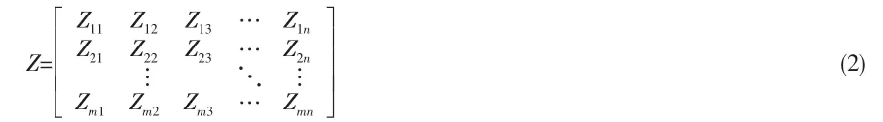
where m is the number of strain sensors used in the full-scale measurement and n is the number of discretized pressure areas of the model.The element Zijis derived by applying the unit load puniton each pressure area j.The equation of element Zijis

or

where γijand εijare shear and normal strains of sensor i on pressure area j,respectively.

2 Application to a ship

2.1 Agulhas and instrumentation

The Polar Supply and Research Vessel(PSRV)S.A.Agulhas II,which has the ice classPC5[6],was built by STX Finland at the Rauma shipyard and she was delivered in April 2012. The main dimensions of the vessel are shown in Tab.1.

Three areas(bow,bow shoulder and stern shoulder)of the starboard side were instrumented with strain gauges to measure the ice-induced load on the ship hull as presented in Fig.1.This paper focuses on the ice load only on the stern shoulder,the strain data from bow and bow shoulder therefore are ignored here.Eight strain gauges numbered-SS16,SS17,SS18,…,SS23-were located at the frames for measurement of shear strains while the other six strain gauges numbered from SS24 through SS29 at the plate field were used to measure the normal strain.

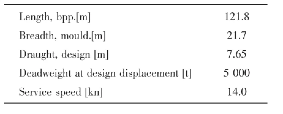
Tab.1 The main dimensions of S.A.Agulhas II

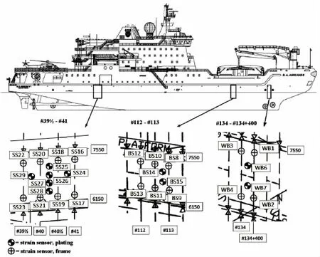
Fig.1 The instrumented areas of the ship hull.From left to right: stern shoulder,bow shoulder and bow[7]

2.2 Load discretization

The classification regulations assumed the ice-induced load area to be rectangular.However,the load pressure distribution is so complicated in reality that it may appear like either lines or spots.Hence the instrumented area was discretized in three different ways to describe the pressure distribution of the ice load[3].Some assumptions also have been made to improve the accuracy of the inverse method by Ikonen.Firstly,the load is perpendicular to the structure and always non-negative(the direction is into structure).Secondly,the ice contact area is a 0.8-meter-strip located in the middle of the two partial platforms,since the design waterline(DWL)is located at the upper partial platform,and the water line was a little below the DWL during the voyage.Furthermore,the strip is narrowed into 0.622 meter due to most likely the load is going to be inside this narrower area.

Fig.2 presents the first discretization consisting of 8 individual fixed ice pressure areas. Discretization 1 aims to minimize the function with a simple and robust way to save the calculation time.

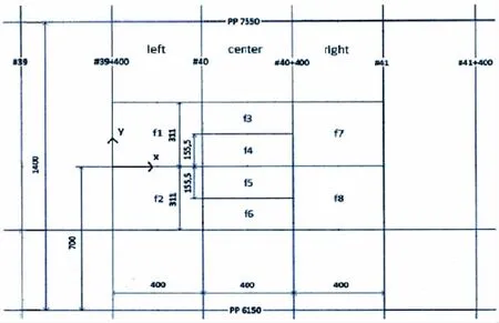
Fig.2 Discretization 1,all dimensions are in millimeters

There are 20 individual fixed ice pressure areas in the discretization 2 as shown in Fig.3. The purpose to have more pressure areas is to increase the accuracy of the pressure distribution.

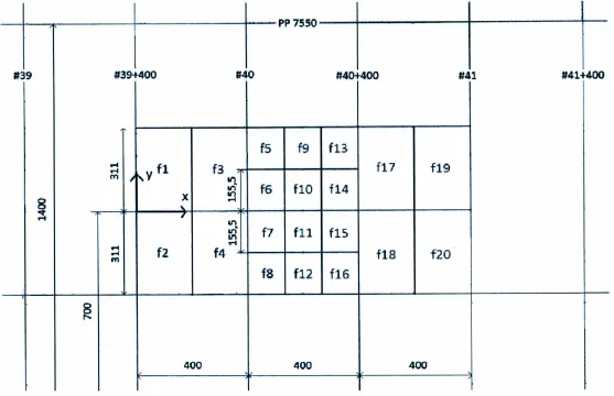
Fig.3 Discretization 2

Discretization 3(Fig.4)is a portion of discretization 2 with assumption that the load to bemainly fall onto the center of frame span.Therefore the strain data from sensors SS16,SS17, SS22,SS23,SS24 and SS29 will be ignored.The third discretization is used to compare the loads on plate fields and frame.

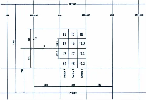
Fig.4 Discretion 3

2.3 Finite element method(FEM)

The software FEMAP(version 11.0) was employed in building the finite element model consisting of 38198 triangular and quadrilateral elements in total. The inner and outer sides of the model are presented in Figs.5 and 6 within which the fine mesh on central area implies the instrumented area.To improve the efficiency of analysis,some geometrical details,such as lightening holes wereignored to reduce the number of element in FEM model.As shown in Fig.7,all translational and rotational of displacements are fixed at the boundaries marked by the blue triangles,and the instrumented area is far away from the boundaries to eliminate the influence of borders.

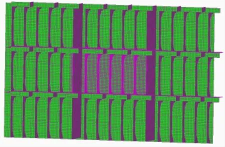
Fig.5 FEM model from the inner side of the hull

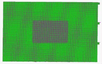
Fig.6 FEM model from the outer side of the hull

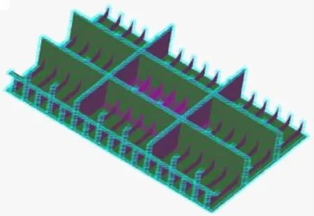
Fig.7 Boundary conditions of the Finite element model

3 Verification

3.1 Verification of inverse method

The ice-induced load distribution is virtually complicated and cannot be exactly reflected by the discretized pressure areas.7 cases are considered in this paper investigating how the method works in different loading situations.Only the third discretization was tested here since it has the simplest form that all the pressure areas are in the same size and located in the center frame span.The initial pressure for each case was set to 1 000 Pa for simplifying further analysis.

The procedure of validation is illustrated in Fig.8.

3.1.1 Assumption cases

The case 1 shown in Fig.9 is to apply ice load p individually on each pressure area of discretization 3.This is the ideal situation,whose results should match the input exactly to validate the algorithm’s correctness.

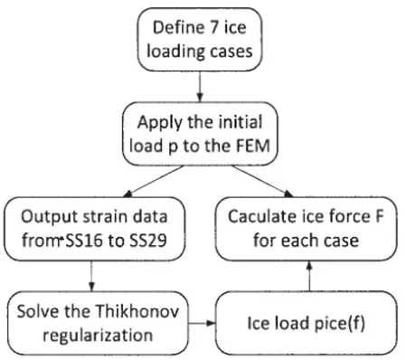
Fig.8 Procedure of the validation

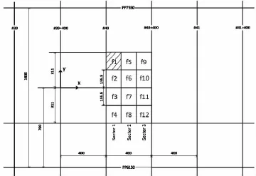
Fig.9 Case 1

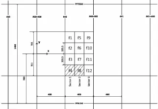
Fig.10 Case 2

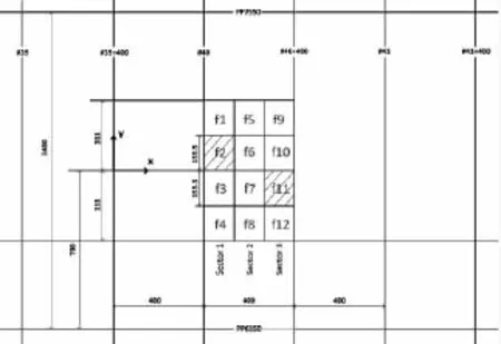
Fig.11 Case 3

In case 2(Fig.10),the loading area is two adjacent pressure areas(f4&f8)and the case3 (Fig.11)also has two pressure areas,but they are non-adjacent(f2&f11).The aim of these two cases is to estimate the results when a loading area is not only one facet.

In case 4(Fig.12),the loading area is a portion of two adjacent discretization areas(in the center of f2&f6).Then the loading area will be extended to four pressure areas(in the center of f1,f2,f5&f6)in case 5(Fig.13).The purpose of these two cases is to determine whether the boundaries affect ice load distributions.

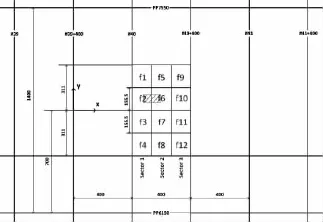
Fig.12 Case 4

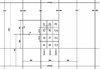
Fig.13 Case 5

The case 6(Fig.14)simulates the situation when ice loads are outside the discretization areas,but still in the center frame span(below f8&f12).And in the case 7(Fig.15),the ice loading area is outside the frame(case7.a,on the left of f8&f12)or through the frame(case7.b, in f11 and extend outside).The goal of these two cases is to estimate whether the model can handle outside loading and present its impact on the model.

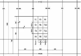
Fig.14 Case 6

3.1.2 Results of load distribution and forces

Case 1 described the ideal situation,where loading area is the same as the single pressure area.Perfect results are gotten in this case:the pressure distributions are exactly as the same as the initial ones.Fig.16 illustrates only two results of case 1,since the others are similar.

As shown in Fig.17,the load distribution of case 2 is as the same as the input one,but the pressure value of f4 is greater than that of f8.In case 3(Fig.18),both the distribution areasand pressure values are changed.Even-though some pressure occurred on unloaded areas,their values are very small.

Fig.16 Ice load distribution of case 1,the loading area is f1(a)and f2(b),respectively

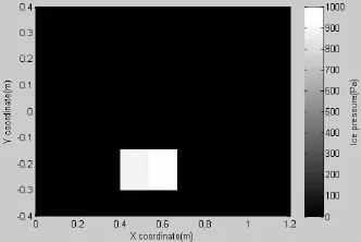
Fig.17 Ice load distribution of case 2

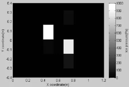
Fig.18 Ice load distribution of case 3

The results of case 4(Fig.19)and case 5(Fig.20)seem good,the distribution areas accuracy and the pressure values turn down due to initial load did not fill the pressure areas.The values in four pressure zones of case 5 are not the same,since the input load is not at the center of the four pressure areas.

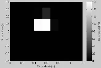
Fig.19 Ice load distribution of case 4

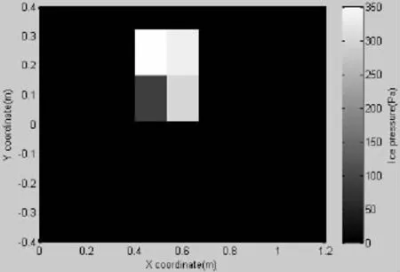
Fig.20 Ice load distribution of case 5

The result of case 6(Fig.21)presents only one load pressure area,even-though the initial loading area is two facets(below f8 and f12).Obviously the frame#40+400 closed to thepressure area f12 affects the load distribution.

The influence of fames is more obvious in case 7(a)since the ice loads are applied outside the frames.As can be seen from Fig.22, the pressure values are extremely small and the load distribution does not follow the assumption.The result of case 7(b)is better than that of case 7(a)due to the loading area including one discretized pressure area.

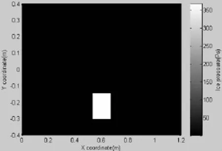
Fig.21 Ice load distribution of case 6

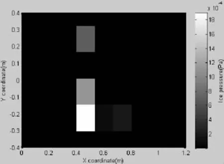
Fig.22 Ice load distribution of case 7(a)

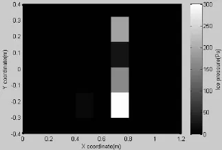
Fig.23 Ice load distribution 7(b)

3.1.2 Ice force

Result errors cannot be estimated with pressure values from above figures because the load distribution areas are not the same as previous.Hence ice forces are compared for accuracy and intuitionistic results.

Comparison of the initial ice forces and calculation ice forces based on inverse method for each case is presented in Tab.2.

As can be seen from Tab.2,the errors are below 2%for cases1,2 and 3.This means perfect results can be reached when the loading areas have the same sizes as the discretized pressure areas.However,it rarely happened in reality.In cases 4 and 5,the errors increased to almost 9%because the boundaries of pressure areas affect results,but they are acceptable in engineering problems.From cases 6 to 7,the errors are above 50%,which are not allowed.As it was expected,the model cannot handle the situation,when the ice loads are outside the discretization areas.

3.2 Case study

3.2.1 Measurement data

The voyage from Cape Town(South Africa)to Antarctica started on 28th November,2013and ended 13th February,2014.During the whole voyage,the ice was observed between 7th December and 1st February with the maximum thickness over 1.0 m,which is thicker than the designed ice thickness of S.A.Agulhas II.The mechanical properties of sample ice with 1.75 m in thickness are described in Tab.3.The ice conditions were relatively severe to the vessel in Antarctica.

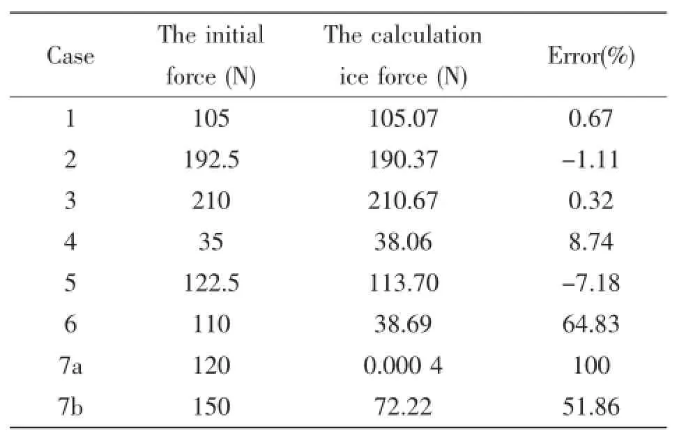
Tab.2 Comparison of the initial and calculation ice force

Usually the ice loads occur on the stern shoulder when the ship breaks out of a channel or turns in level ice.Two typical ice contacts-starboard ram and following a brash channelwere selected for further analysis.The observed ice thickness was mainly between 0.2 m and 0.25 m during these two ice contacts.The strain data of ice contacts is presented in Fig.24 and Fig.25.

Tab.3 Mechanical properties of 1.75 m ice during the voyage[8]

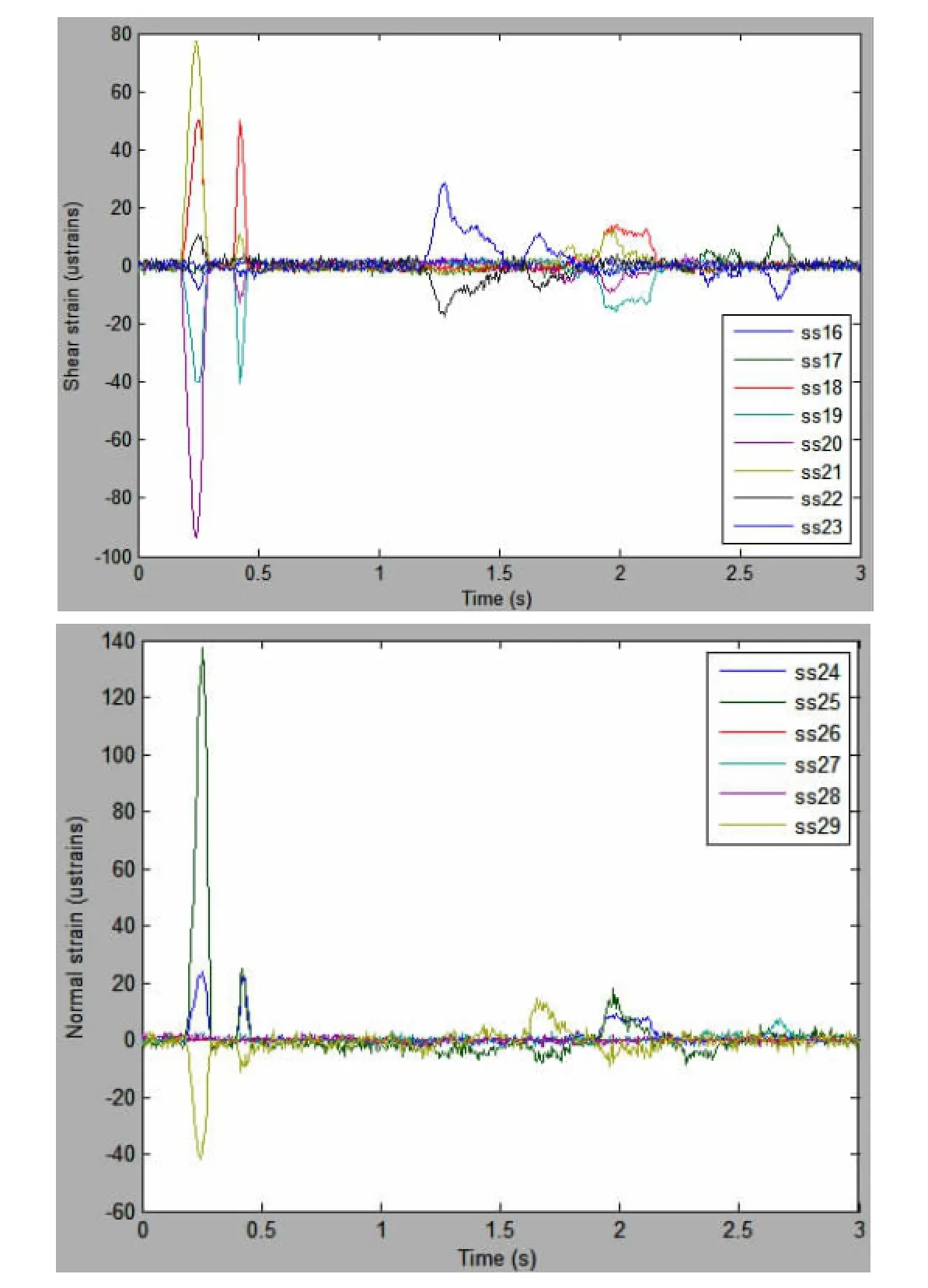
Fig.24 Shear and normal strains of starboard side ram

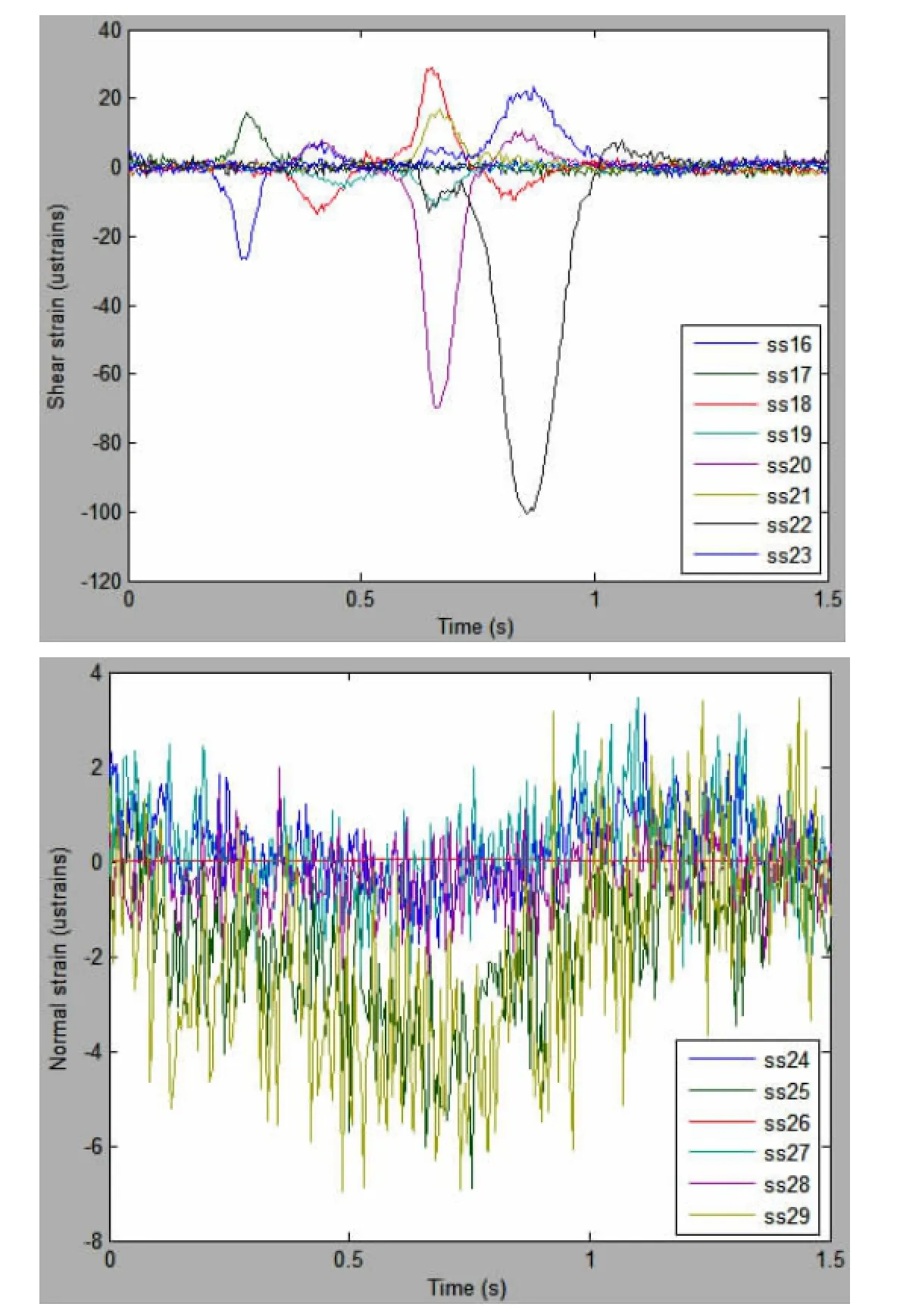
Fig.25 Shear and normal strains of following a brash channel

3.2.2 Results of measurement data

Only the ice load in the center frame span will be calculated due to most of the strain sensors are located at the central areas.The equations of ice loads by all the three discretization are:

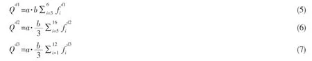
where a=155.5 mm and b=400 mm as in Fig.2.The superscripts,d1,d2 and d3,refer to discretization 1,discretization 2 and discretization 3,respectively.

Fig.26 presents the ice loads in the center frame span of starboard ram,where strain data was shown in Fig.24.The peak load of all three discretization occurred at 0.26 s in common, while the largest value is almost 35 kN based on discretization 3 and the smallest is 27 kN ofdiscretization 2.Discretization 1 also shows a second peak after 0.06 s, which is about 6 kN.

The ice loads of following a brash channel(the same case as presented in Fig.25)are shown in Fig.27.Discretization 2 could not work in this ice contact due to the failure of optimizing algorithm.The peak loads determined by discretization 1 and 3 are similar-they both occurred at 0.6 s and the value is around 15 kN.But there are some small waves in the load line of discretization 1 before 0.3 s and after 0.8 s.According to case 6 and case 7 in Section 3.1,discretization 3 could not be easily affected by the outside loading of the central frame span.This means that the ice load not only occurred in the center frame span,but also nearby the central areas when the vessel navigated in a brash channel.

Since the results of ice load by discretization 2 are quite different from those of discretization 1 and 3,the second discretization will be ignored for further analysis.The ice load distribution of the whole instrumented area can be determined by discretization 1.However,the result is rough due to the less number of discretized areas.This disadvantage can be overcome by discretization 3,which has more discretization variables.Fig.28 presents ice load distributions of starboard ram-the peak load from Fig.26-with discretization 1 and discretization 3,while the ice load distributions in Fig.29 refer to the peak load of following a brash channel (as shown in Fig.27).

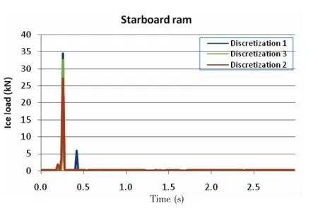
Fig.26 Ice load of starboard ram

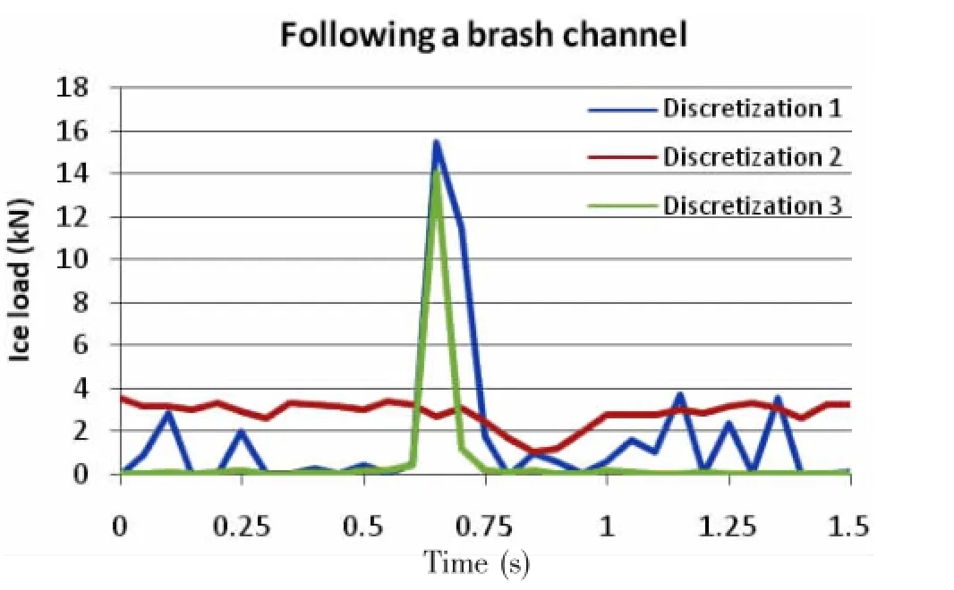
Fig.27 Ice load of following a brash channel

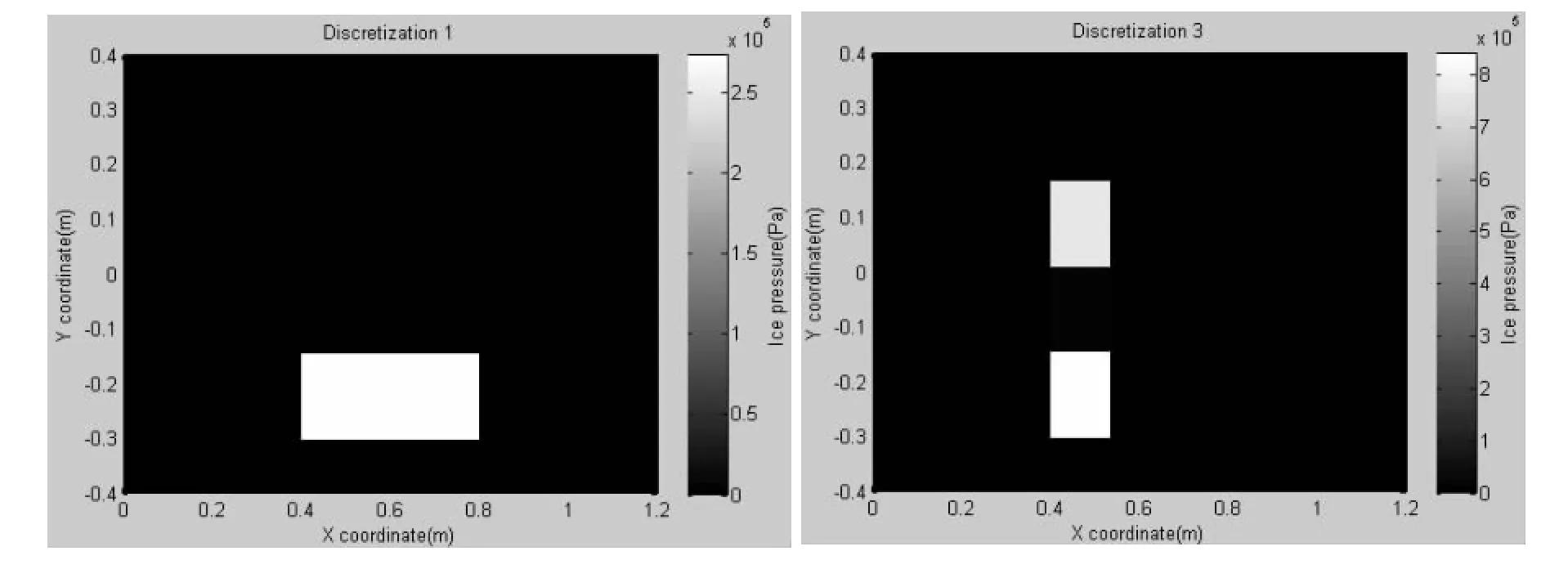
Fig.28 Pressure distributions of starboard ram determined by discretization 1 and discretization 3

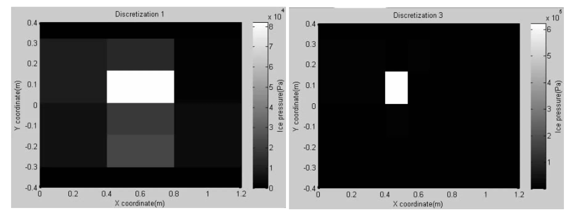
Fig.29 Pressure distributions of following a brash channel determined by discretization 1 and discretization 3

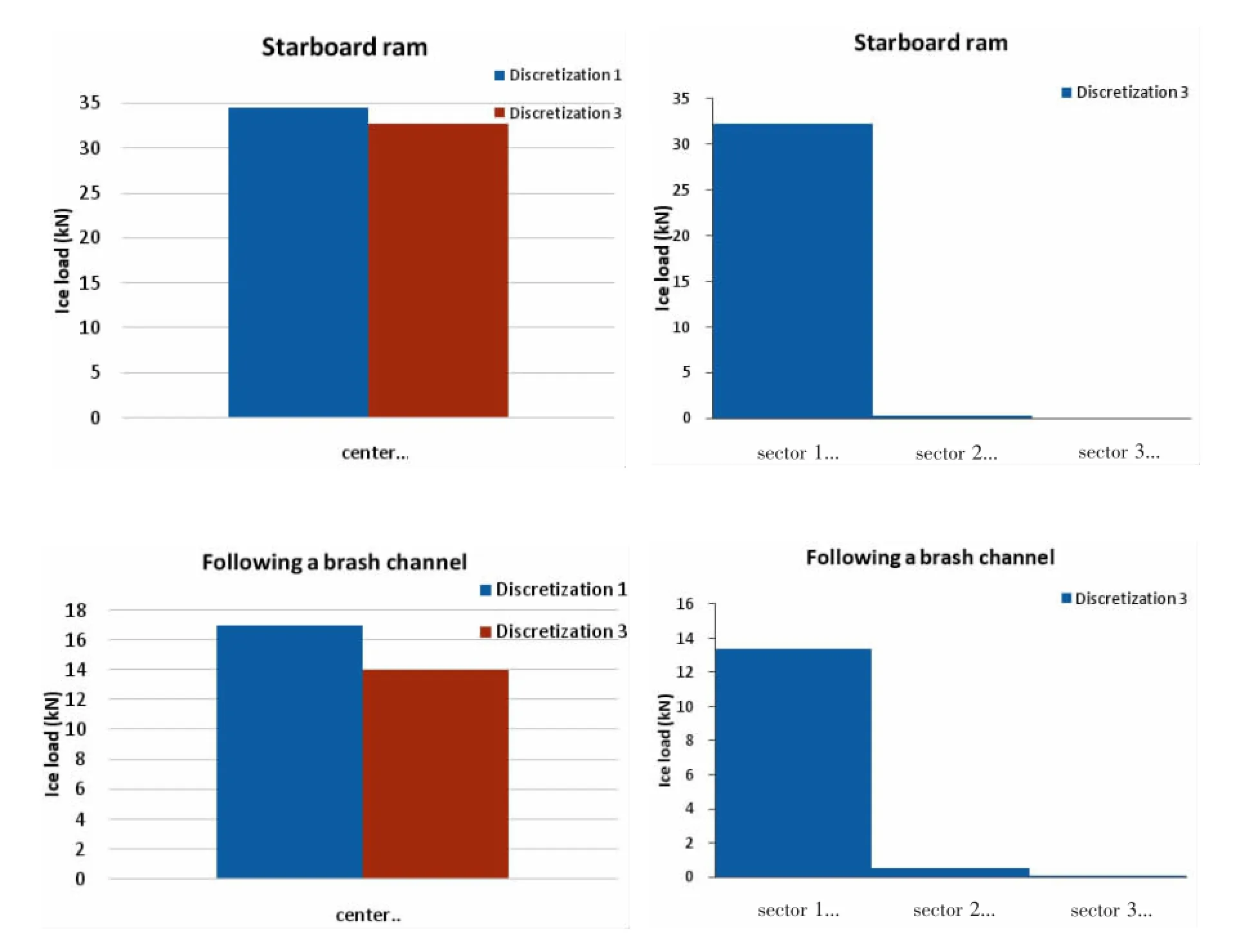
Fig.30 Horizontal location of ice load by discretization 1 and 3

As can be seen from Figs.28 and 29,the similarities for the both ice contacts include that peak load is located at the central frame span and some smaller pressures are visible in the left frame span.It is worth noting that the pressure magnitude of discretization 3 is ten timesbigger than that of discretization 1 in Fig.29.Since the ice load acted mainly on the central area,the horizontal and vertical locations of peak load in the center frame span are presented from Fig.30 to Fig.31.Where center corresponds to the center frame span in Fig.4,sectors 1, 2 and 3 are the portions of center frame span in Fig.6.

Discretization 1 divided the instrumented area into 3 portions in horizontal direction,and the center frame span was separated into 3 parts by discretization 3 further.So only the center part of discretization 1 was presented to compare with discretization 3.As can be seen from Fig.30,firstly the load values determined by discretization 1 are about 2 kN bigger than discretization 3,secondly all peak loads were located at the left sector of central frame span,while the ice loads sharply decreased in the middle sector and kept turn down to the right side.

In the vertical direction,discretization 1 and discretization 3 consist of four areas in the center frame span.As Fig.31 shows,when starboard ram occurred,the ice load determined by discretization 3 acted mainly on the strip whose height is from-155.5 mm to 0 mm,while discretization 1 divided the load into two areas between-311 mm and 0 mm.The similar distributions of vertical location of ice load are gotten in discretization 1 and discretization 3 when the vessel navigated in a brash channel.The ice loads were mainly located at the strip whose height is from 0mm to 155.5 mm,and the ice loads were so small that could be ignored in other heights of the center.

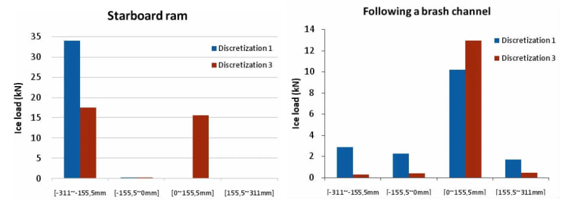
Fig.31 Vertical location(y coordinate)of ice load by discretization 1 and 3

4 Conclusions

Thikhonov regularization was selected as the inverse method to solve the ice-induced loads on stern shoulder of the ship with full-scale measurement data of the voyage in Antarctica.Although three kinds of discretization were considered to form the natural features of ice load,one of them did not work,while the other two gave the similar results.According to the 3rd chapter,verification of the inverse method,results of the model are reliable if the ice-induced load occurred in the discretized pressure areas.As shown from the results of measurement data,ice load nearby the center frame span had more impact on ice load distribution ofdiscretization 1 than discretization 3.

Two patterns of ice contact are considered in this paper.The results presented that all peak loads appeared at the center frame span and the loading area is not bigger than one pressure area of discretization 3.Therefore,more discretization variables could be used to improve the accuracy of results in further analysis.

[1]Uhl T.The inverse identification problem and its technical application[J].Archive of Applied Mechanics,2007,77:325-337.

[2]Romppanen A.Inverse load sensing method for line load determination of beam-like structures[D].Finland:Tampere U-niversity of Technology,2008.

[3]Ikonen T.Inverse ice-induced load determination on the hull of an ice-going vessel[D].Finland:Aalto University,2013.

[4]Thikhonov A,Arsenin V.Solution of ill posed problems[M].Washington DC:Winston and Sons,1977.

[5]Inoue H,Harrigan J,Reid S.Review of inverse analysis for indirect measurement of impact force[J].Applied Mechanics Reviews,2001,54(6):503-524.

[6]Requirements concerning polar class[S].International Association of Classification Societies(IACS),2011.

[7]Suominen M,et al.Full-scale measurements on board PSRV S.A.Agulhas in the Baltic Sea[C]//Pro-ceedings of the 22nd International Conference on Port and Ocean Engineering under Artic Conditions.Espoo,Finland,2013.

[8]Kujala P,Kulovesi J,Lehtiranta J.Full-scale measurements on board S.A.Agulhas II in the antarctic waters 2013-2014 [R].Finland:Aalto University,2014.

基于反向方法的船體冰載荷研究

劉瀛昊1，SUOMINEN Mikko2，KUJALA Pentti2

（1.哈爾濱工程大學(xué)船舶工程學(xué)院，哈爾濱150001；2.阿爾托大學(xué)應(yīng)用力學(xué)系船舶技術(shù)實(shí)驗(yàn)室，芬蘭15300）

船舶碰撞海冰引起的冰載荷分布是十分復(fù)雜的。文章選取Thikhonov正則化這一反向方法，根據(jù)極地科考補(bǔ)給船S.A Agulhas II號(hào)于2013-2014年間南極航行時(shí)實(shí)測(cè)的數(shù)據(jù)，分析得到了船體艉肩部的冰載荷。通過應(yīng)用三種獨(dú)立的冰載荷離散方式來模擬海冰的自然特性，在有限元中得到模型的影響矩陣，并應(yīng)用Matlab對(duì)Thikhonov正則化方程進(jìn)行了優(yōu)化。研究結(jié)果表明，反向方法可以克服數(shù)據(jù)處理過程中的不適定性，并計(jì)算得到船體冰載荷。

冰載荷；有限元方法（FEM）；Thikhonov正則化；載荷離散；反向方法

U661.4

A

劉瀛昊（1988-），女，哈爾濱工程大學(xué)船舶工程學(xué)院博士研究生；SUOMINE Mikko（1985-），男，芬蘭阿爾托大學(xué)博士研究生；KUJALA Pentti（1954-），男，芬蘭阿爾托大學(xué)教授。

U661.4 < class="emphasis_bold">Document code:A

A

10.3969/j.issn.1007-7294.2016.12.010

1007-7294（2016）12-1604-15

Received date：2016-07-15

Biography：LIU Ying-hao(1988-),female,Ph.D.candidate of Harbin Engineering University,E-mail: B412010010@hrbeu.edu.cn;SUOMINE Mikko(1985-),male,Ph.D.candidate of Aalto University, E-mail:mikko.suomine@aalto.fi;KUJALA Pentti(1954-),male,professor of Aalto University, E-mail:pentti.kujala@aalto.fi.