DNS Study on Volume Vorticity Increase inBoundary Layer Transition

Wang Yiqian, Tang Jie, Liu Chaoqun*, Zhao Ning

1.College of Aerospace Engineering, Nanjing University of Aeronautics and Astronautics, Nanjing 210016, P.R. China;2. Department of Mathematics, University of Texas at Arlington, Texas 76010, USA

(Received 15 January 2016; revised 20 February 2016; accepted 5 March 2016)

DNS Study on Volume Vorticity Increase inBoundary Layer Transition

Wang Yiqian1, Tang Jie2, Liu Chaoqun2*, Zhao Ning1

1.College of Aerospace Engineering, Nanjing University of Aeronautics and Astronautics, Nanjing 210016, P.R. China;2. Department of Mathematics, University of Texas at Arlington, Texas 76010, USA

(Received 15 January 2016; revised 20 February 2016; accepted 5 March 2016)

The issue whether transition from laminar flow to turbulent flow on a flat plate should be characterized as a vorticity redistribution process or a vorticity increasing process is investigated by a high-order direct numerical simulation on a flat plate boundary layer. The local vorticity can either increase or decrease due to tilting and stretching of vortex filaments according to the vorticity transport equation while the total vorticity cannot be changed in a boundary layer flow in conforming to the F?ppl theorem of total vorticity conservation. This seemingly contradictory problem can be well resolved by the introduction of a new term: volume vorticity of a vorticity tube, defined as vorticity flux timed by the vorticity tube length. It has been shown that, although vorticity flux must keep conserved, the total volume vorticity is significantly increased during boundary layer transition according to our direct numerical simulation (DNS) computation, which directly results from the lengthening (stretching and tilting) of vortex filaments. Therefore, the flow transition is a process with appreciable increase of volume vorticity, and cannot be only viewed as a vorticity redistribution process.

volume vorticity; vorticity redistribution; vorticity increase; transition; boundary layer

0　Introduction

The creation, redistribution and conservation of vorticity have been studied extensively in vorticity dynamics with a long history[1-4]. It is found that vorticity cannot be generated nor destroyed within the interior of fluids, and is transported by advection and diffusion in two-dimensional flows[5]. For a three-dimensional flat plate boundary layer flow, the F?ppl theorem[1]holds and the total vorticity is constant. Based on these facts, it is believed that the transition from laminar flow to turbulence is mainly a vorticity redistribution process.However, some university lecture notes[6]emphasize that the local vorticity could be intensified (or diminished) according to the vorticity transport equation, especially at the location of coherent structures in turbulent flows. Therefore, flow transition cannot be only assumed as a vorticity redistribution process, but also, and more importantly, a vorticity increase process.

Although vorticity generation, especially at boundaries, has been widely investigated analytically and numerically in the two-dimensional flows[7-10], few research has been found regarding to vorticity dynamics numerically in three-dimensional turbulent flows.Wu[11]discussed interfacial vorticity dynamics in three dimension. And studies on vorticity distribution in boundary layer flow can also be found in the literature[12-14]. However, the variation of total vorticity in a boundary layer has not been addressed. In order to answer the questions of whether total vorticity is increased and whether vorticity flux is conserved in a transitional boundary layer flow and if it is appropriate to call transition a redistribution process, a high fidelity direct numerical simulation (DNS) was conducted on a boundary layer flow[14-15]. Based on the data obtained, we have gained some insights on this issue.

1　Vorticity Dynamics

1.1The first Helmholtz vorticity theorem

It is easy to verify that vorticity has zero divergence, i.e.ω=0, which leads to

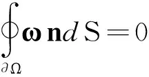
(1)

where n is the outward pointing unit vector and ?Ω represents a closed surface in space. Eq.(1) means the integration of vorticity flux over any closed surface in a single domain must be zero. Thus, for a vorticity tube, the integrated vorticity flux over any cross surface must be the same, which is referred as the first Helmholtz vorticity theorem.The computational domain of our DNS is shown in Fig. 1 and the initial laminar flow condition is obtained by solving the Blasius equation. Therefore, all the vorticity lines inside the computational domain are straight lines starting from the right side boundary S1 and ending at the other S2. Thus, the amount of vorticity tubes passing through any cross section normal to spanwise direction is exactly the same. In addition, every vorticity tube has the same vorticity flux based on the first Helmholtz theorem. Then the vorticity flux for these sections must be constant, which equals exactly to the side boundary vorticity flux, i.e.

(2)

where S is any cross section plane and j the spanwise unit vector.

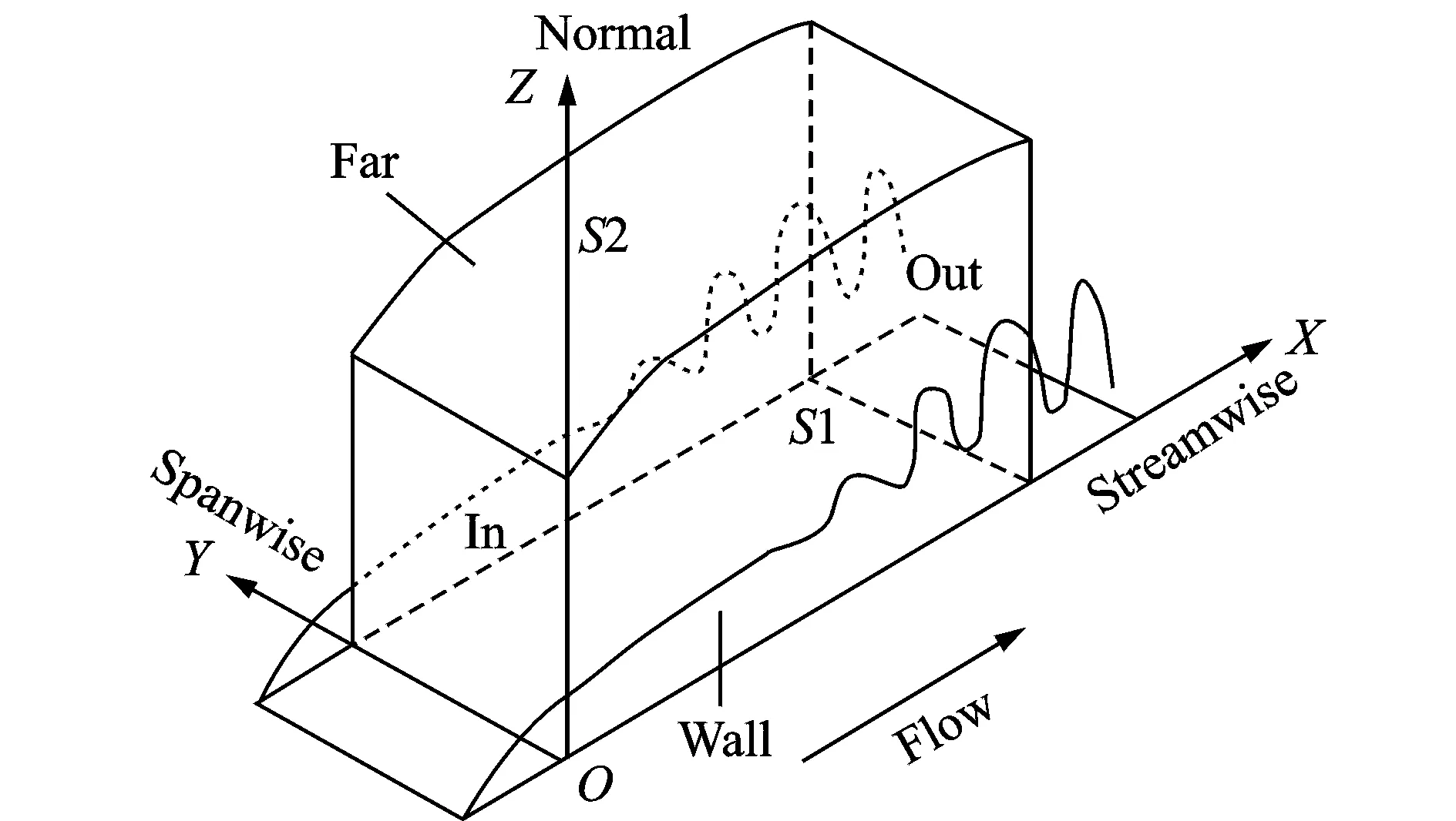
Fig.1　The computational domain

Disturbances (i.e. Tollmien-Schlichting waves) are enforced at the inflow boundary during the simulated transition process. However, little vorticity is introduced into the flow domain due to T-S waves since they are in orders smaller than the main flow. On the other hand, vorticity lines must end on boundaries, except for self-closed vorticity lines according to the theorem. However, only a small amount of closed vorticity lines are found during the simulation. Therefore, most vorticity lines during transition originate from one side boundary and end at the other one. As stated above, we have a formula which should hold for the whole transition from laminar flow with Blasius solution to turbulence for any sections normal to the spanwise direction.

∫Sω·jdS≈const

(3)

Next, the integration of vorticity over the whole computational domain Ω is considered.

(4)

where ?Ω is the surface of Ω, r the position vector while S1, S2, In, Out, Wall and Far refer to the side, inflow, outflow, wall and far field boundaries, respectively, as shown in Fig. 1. Since vorticity ωyis dominant and ωxat the inflow and outflow boundaries is in orders smaller, then

(5)

where b is the spanwise length of the computational domain.Therefore, the integral of the spanwise vorticity ωyover the whole domain approximately equals to the integral of ωyover any cross section plane timed by spanwise length. As Eq.(3) indicates, ∫Sω·jdS is nearly a constant for any cross section at a given time. Actually, ∫Sω·jdS does not change from time to time during the transition process based on the DNS results, which will be presented in the next section. Therefore, ∫ΩωydV does not change much as time changes, i.e.

(6)

(7)

1.2Vorticity transport equation

In the case of incompressible and Newtonian fluids,the vorticity equation can be written as

(8)

where ν is the kinematic viscosity, V the velocity vector and the equation is called vorticity transport equation. The second term on the right-hand side of Eq.(8) accounts for diffusion of vorticity due to viscous effects. For a two-dimensional flow: V=(u,v,0),ω=(0,0,ω).Thus, the first term on the right-hand side vanishes. The equation turns into an advection-diffusion type equation, which naturally leads to a conclusion that the vorticity can spread by diffusion, and be moved by advection, but the total vorticity (integral of vorticity over the domain)is conserved for all localized blobs of fluids. For three-dimensional flow, the first term (ω·)V is of great importance. It represents the stretching or tilting of vorticity due to the flow velocity gradients, which means the local vorticity could be increased or decreased.

1.3Volume vorticity of a vorticity tube

In order to better explain the issue, we now introduce the so-called volume vorticity. Imagine a point P in the flow field. Then a vorticity line passing through the point can be found as Fig. 2 shows, and an infinitesimal vorticity tube can be drawn around the vorticity line. The volume vorticity of a vorticity tube is defined as

(9)

where V and L represent the volume and length of a vorticity tube, and n, A have the same direction as local vorticity. Fcis the cross vorticity flux and stays constant for a given vorticity tube. Thus,

(10)

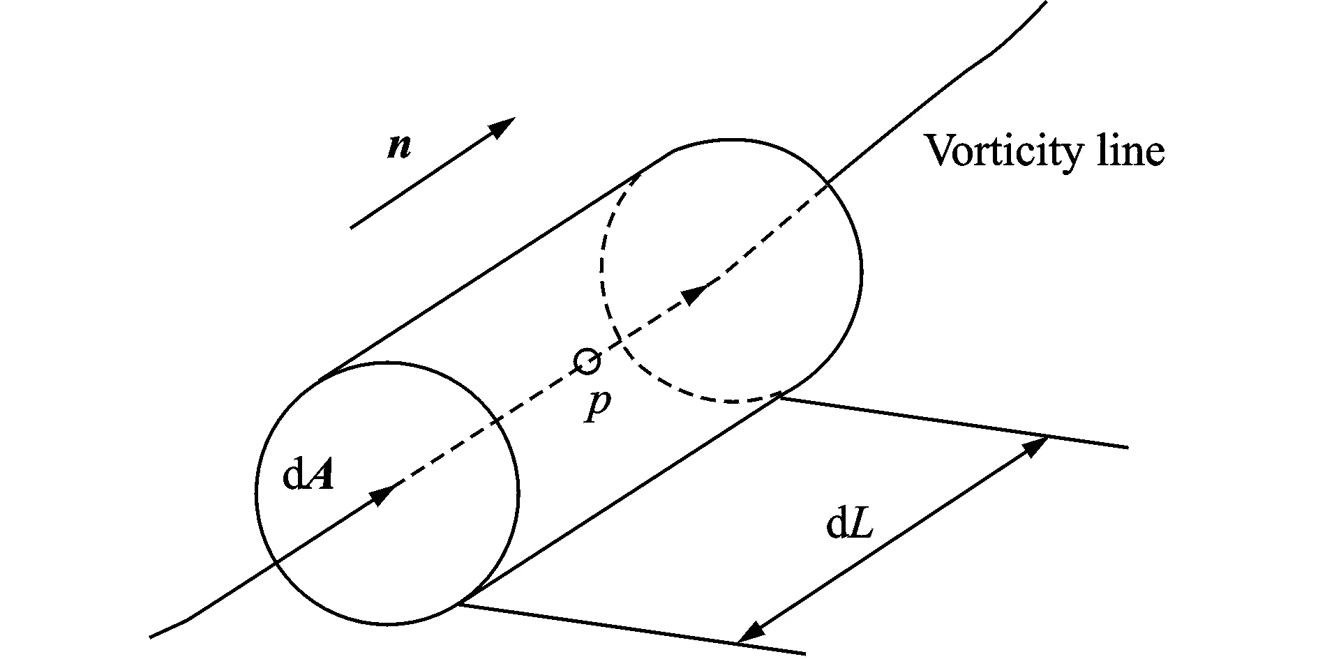
Fig.2　The computational domain

Eq.(10) implies that, for a given vorticity tube, which has a constant cross section vorticity flux Fc, the volume vorticity ωVis determined by the length of the vorticity tube.For a laminar boundary layer flow with Blasius solution, the volume vorticity of a vorticity tube is minimized since all vorticity lines are straight lines starting from one side boundary and ending at the other. By tracking vorticity lines during the transition process, it is found that the vorticity lines are lengthened by tilting, stretching and twisting, which will lead to significant volume vorticity increase. Therefore, the volume vorticity could be a good symbol of turbulence strength, and an indication of transition stage.

The integration of volume vorticity over the side boundary S1 is

(11)

where ω is the magnitude of vorticity vector.And since all the vorticity lines start and end at side boundaries except for self-closed vorticity lines, which are much weaker, for boundary layer flow, the integral can be further written as

(12)

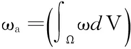
Therefore, the integral of vorticity magnitude over the whole computational domain represents the integral of the volume vorticity of all vorticity tubes inside the flow. In addition, we introduce another term of average volume vorticity, which can be used to represent to what extent the concerned area become turbulent, i.e.

ωa=(∫ΩωdV)/Ω

(13)

2　DNS Analysis

In this section, we analyze the DNS data to verify the conclusions derived in the previous section, and try to take advantage of volume vorticity and average vorticity to illuminate the issue whether transition from laminar to turbulent flow should be characterized as a vorticity redistribution process.

2.1Vorticity flux conservation

The vortical structures at t=7.88T (T is the period of the T-S wave) from the DNS results are shown using theΩ-vortex identification method[16]in Fig.3, which is a typical time step of the transition process.

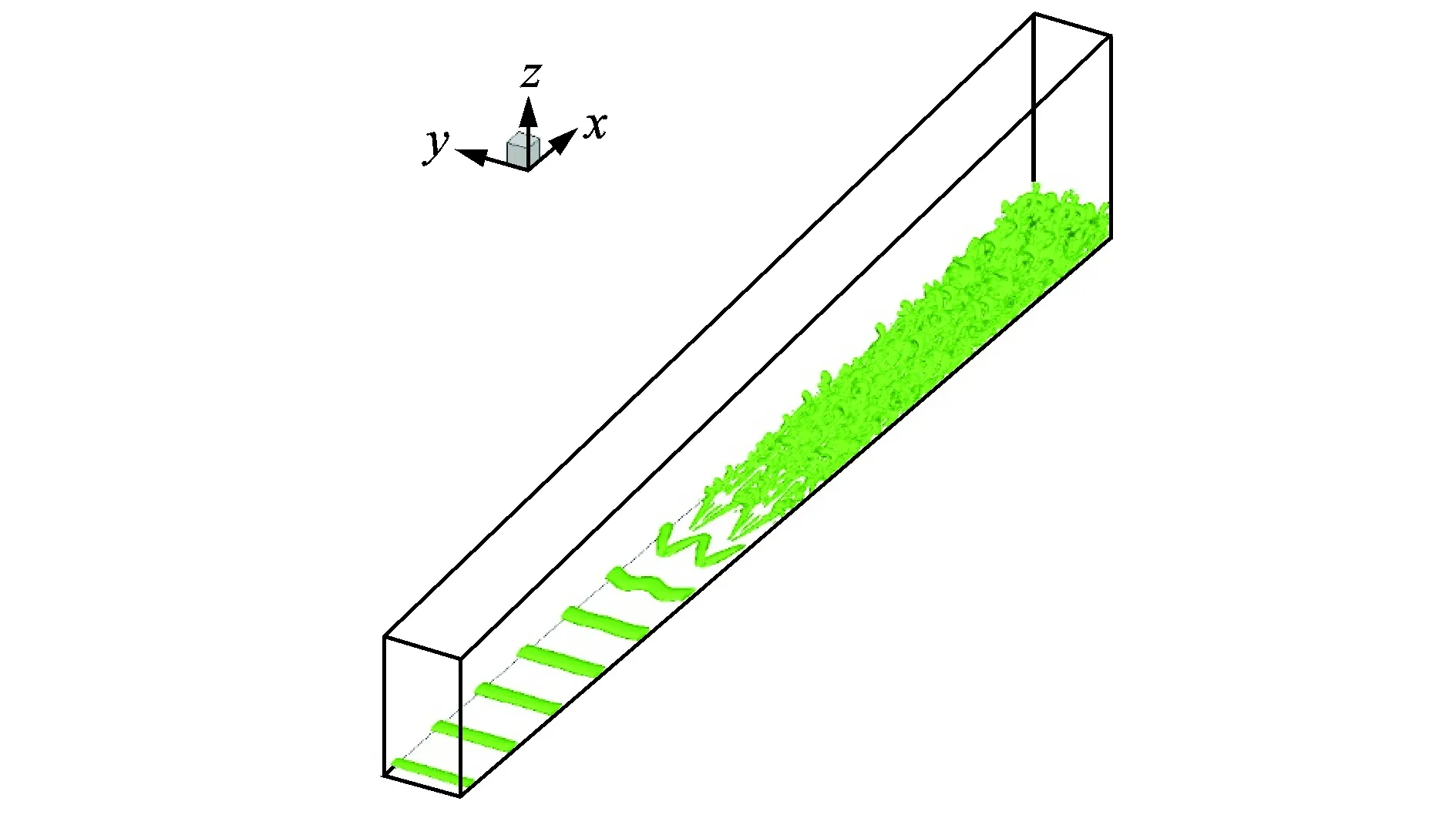
Fig.3　Vortical structures at t=7.88T

For sections normal to spanwise direction, it has been concluded ∫Sω·jdS≈const (Eq.3). The integrals over five sections including two side boundaries are listed in Table 1. Similar results can be obtained from other time step in the DNS data. These results confirm that the vorticity flux is conserved as expected.

2.2Spatial integral of vorticity

From Table 2, it can be seen that the integrals ofωxandωzare always around zero, and ∫ωydV is nearly conserved at different time steps while the vortical structures at the corresponding time steps are quite different as shown in Figs.3，4. In addition, the relation depicted by 2 is confirmed by the DNS results.

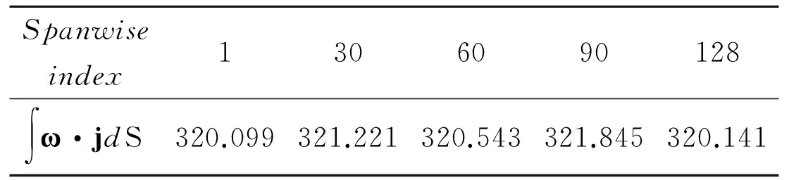
Table 1　Vorticity flux over cross sections

Table 2　Integral of vorticity over the computational domain at different time steps

Fig.4　Vortical structures

From the above analysis, it is clear that the vorticity flux conservation law cannot be violated and the integral of the vorticity vector over the whole domain conserves even the transition happens and numerous vortical structures have built up.

2.3Volume and average vorticity development during transition

The conception of volume vorticity is introduced to more accurately depict the transition process. Since the average vorticity is easier to obtain, Table 3 shows the results at t=4.30T, 6.09T and 7.88T.

From the data in Table 3, it is clear that the average vorticity significantly increased during the transition process. Next, we will try to take advantage of the notion of volume vorticity to explain why the average vorticity significantly increases while the integration of vorticity vector conserves during the transition process. In order to demonstrate the volume vorticity can be significantly increase, several examples are given.

Fig.5 (a) shows a randomly selected vorticity line near the flat plate in Blasius solution. Here,ωx=ωz=0, and the vorticity line is straight starting from one side boundary and ending at the other. If we imagine a vorticity tube around this vorticity line, the cross section area should be the same since vorticity flux has to be conserved. From Fig. (b), it can be seen that vorticity rollup (tilting and stretching) happens in aΛvortex. The vorticity flux of the vorticity tube must keep conserved while the vorticity magnitude has been changed shown by the contour in Fig.5 (b). Therefore, the color on the vorticity line could also be viewed as a symbol of the cross section area of the imagined vorticity tube (large vorticity magnitude means small section area and vice versa). By comparing Figs. 5 (a),(b), it is clear that the volume vorticityωVhas been increased since the vorticity tube is lengthened due to vorticity tilting and stretching.

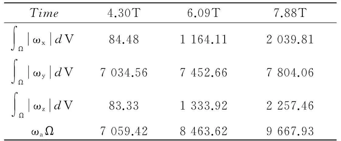
Table 3　Vorticity components and magnitude integrals over the whole domain

Fig.5　Typical vorticity lines

In addition, we now consider the integration of vorticity vector over the vorticity tube in Fig.5(b). Fig.6 shows the distribution of streamwise and normal vorticity which exist in the Blasius solution.Bothωxandωzappear as positive and negative values, and the symmetry obviously leads to ∫ωxdV=∫ωzdV=0 for a given vorticity tube. Therefore the integration ofωxandωzover the whole computational domain should be around zero since they approximately equal the summation of ∫ωxdV and ∫ωzdV over side boundary. The approximation mainly comes from the inlet and outlet boundary,where vorticity tubes might end.

Fig.6　Streamwise and normal vorticities distribution

In conclusion, any vorticity tube should have only one section vorticity flux but different volume vorticity depending on the length of the vorticity tube during a transition process.It clearly shows that if the vorticity line surrounded by a small vorticity tube is twisted or stretched, the length of the tube will increase thus leading to the volume vorticity increase. In the laminar Blasius solution, all vorticity lines are straight lines starting from one side boundary and ending at the other, which should be the minimized volume vorticity and therefore the minimum average vorticity for the whole domain. Those vorticity lines will be twisted and stretched during flow transition. Consequently, the vorticity tubes would become longer and longer and the volume vorticity becomes larger and larger although the vorticity flux in any vorticity tube must keep conserved. It can be found that ∫ΩωxdV≈0,∫ΩωzdV≈0 and ∫ΩωydV is nearly a constant (Table 2).However, we believe the volume vorticity and the average vorticity can better represent the vorticity distribution since in general we cannot use positive vorticity to cancel or balance the negative vorticity and both are able to drive flow rotation.

Fig.5 (b) shows a very early stage of the transition process. Two more vorticity lines at a later and a much later stage are shown in Fig.7 at t=7.88T. Fig.7 (a) presents a vorticity line passing through a vortex ring. It is shown the vorticity line is further twisted and stretched. Therefore, the volume vorticity has become larger since the vorticity tube has a larger length. Fig.7 (b) shows a much later vorticity line which has become very long since it has been twisted many times. In addition, the vorticity line in Fig.7(b) has lost symmetry, which is a symbol of turbulence.

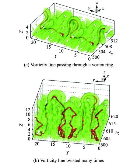
Fig.7　Two vorticity lines at different locations in flow transition at t=7.88T

Another important point that should be addressed is that self-closed vorticity lines exist in the flow field, see Fig.8. These self-closed vorticity lines have no contribution to vorticity flux and integration of vorticity vector over the whole domain. On the other hand, these vorticity lines have non-zero volume vorticity, which will contribute to the increase of average vorticity. However, the closed vorticity tube is not the main source of the volume vorticity increase since the vorticity magnitude at these self-closed vorticity lines is around 0.01, which is in orders smaller than that at the vortical structures.

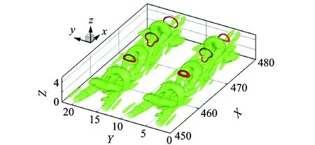
Fig.8　Self-closed vorticity lines at t=4.87T

From the discussion above, the transition process is also a process that the vorticity lines twisted and stretched, and therefore a process of volume vorticity increase. To further verify that the volume vorticity and average vorticity can be symbols of the complexity of the vortical structure, the computational domain at t=7.88T is divided into three sub-domains with same streamwise length as ″early transition zone, transition zone, late transition zone″, see Fig.9.

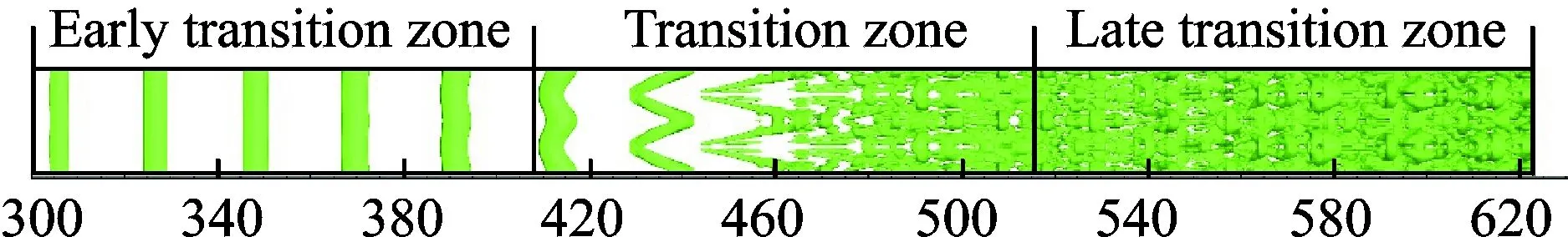
Fig.9　Three subzones with the same streamwise length at t=7.88T

The different vortical structures of three sub-domains with vorticity lines are shown in Fig.10. This indicates that in early transition zone, vortical structures are very simple and vorticity lines are almost straight. In the transition zone, fluid transition starts to occur. Moreover,Λ-vortex, vortex rings and other transition symbols appear while vorticity lines are getting twisted and stretched. Obviously, the length of vorticity lines is increased significantly in this zone. In the last sub-domain, late transition zone, the vortical structures havebecome very complicated. Further twisted and stretched vortcity lines also appear in this domain, whose length increases dramatically. As we discussed above, non-symmetric vorticity line, is found on the late of this zone. Then the flow would finally become turbulent further downstream.

Fig.10　Three subzones with typical vorticity lines at t=7.88T

The calculated average vorticity of three subzones is shown in Table 4. The value of average vorticity is different in the first two zones, but it is much larger in the third zone. Compared with Fig. 10 and Table 4, it is clear that the development of the complicated vortical structure, the growth of vorticity lines in length and the increment of average vorticity values trend to happen simultaneously. Based on this fact, the volume vorticity or the average volume vorticity can be a good symbol of the development of the complexity vortical structure, or the transition stage.

Table 4　The average vorticity of three subzones at　t=7.88T

3　Conclusions

Here we review some basic vorticity dynamics, and apply them to our DNS datasets. The main purpose is to answer the question whether transition should be characterized as a vorticity redistribution process or a vorticity increase process. The conclusions are listed below

(1) Vorticity flux conservation is a law and cannot be violated. As for the DNS case, this means any section normal to the spanwise direction must have same vorticity flux as the side boundary. All vorticity tubes come from the side boundary and they have the same flux along the tube except for those self-closed tubes around low speed zones.

(2) It is true that the local vorticity could be increased or decreased in the flow field during flow transition due to twisting and stretching of vorticity lines, which is quite different from the two-dimensional cases.

(3) If we consider the vorticity in the whole domain,∫ΩωxdV,∫ΩωydV and ∫ΩωzdV are not changed much during the flow transition process. However, considering the sign of vorticity is meaningless because both positive and negative vorticity can drive rotation.

Acknowledgements

This work was supported by Department of Mathematics at University of Texas at Arlington. The authors are grateful to Texas Advanced Computing Centre (TACC) for the computation hours provided. This work is accomplished by using Code DNSUTA released by Dr. Chaoqun Liu at University of Texas at Arlington in 2009. Wang Y.also would like to acknowledge the Chinese Scholarship Council (CSC) for financial support.

[1]F?PPL A. Die geometrie der wirbelfelder [J]. Monatsheftefür Mathematik und Physik, 1897, 8(1):33-33.

[2]LIGHTHILL M J. Introduction: boundary layer theory. In: Laminar boundary theory [M]. Oxford: Oxford University Press, 1963: 46-113.

[3]LUNDGREN T, KOUMOUTSAKOS P. On the generation of vorticity at a free surface [J]. Journal of Fluid Mechanics, 1999, 382: 351-366.

[4]WU J Z, MA H Y, ZHOU M D. Vorticity and vortex dynamics [M].Berlin: Springer Science & Business Media, 2007.

[5]DAVIDSON P A. Turbulence: an introduction for scientists and engineers [M]. 1st Edition. Oxford: Oxford University Press, 2004.

[6]DRELA M. Lecture notes of fluid mechanics and aerodynamics [EB/OL]. [2009-05-04]. http://web.mit.edu/16.unified/www/SPRING/fluids/Spring 2008/LectureNotes/f06.pdf.

[7]MORTON B. The generation and decay of vorticity [J]. Geophysical and Astrophysical Fluid Dynamics, 1984, 28(3-4): 277-308.

[8]WU J Z, Wu J M. Boundary vorticity dynamics since Lighthill′s 1963 article: review and development[J]. Theoretical and Computational Fluid Dynamics, 1998, 10(1): 459-474.

[9]BRONS M, THOMPSON M C, LEWEKE T, et al.Vorticity generation and conservation for two dimensional interfaces and boundaries [J]. Journal of Fluid Mechanics, 2014, 758: 63-93.

[10]ROOD E P. Myths, math and physics of free-surface vorticity [J]. Applied Mechanics Reviews, 1994, 47(6S): 152-156.

[11]WU J Z. A theory of three-dimensional interfacial vorticity dynamics [J]. Physics of Fluids, 1995, 7(10): 2375-2395.

[12]LIU H X, ZHENG C W, CHEN L, et al. Large eddy simulation of boundary layer transition over compressible plate [J]. Transactions of Nanjing University of Aeronautics and Astronautics, 2014, 46(2): 246-251.

[13]SHI W L, GE N, CHEN L, et al. Numerical simulation and analysis of horseshoe-shaped vortex in near-wall region of turbulent boundary layer [J] Transactions of Nanjing University of Aeronautics and Astronautics, 2011, 28(1): 48-56.

[14]LIU C, YAN Y, LU P. Physics of turbulence generation and sustenance in a boundary layer [J]. Computers and Fluids, 2014, 102: 353-384.

[15]LIU C, CHEN L. Parallel DNS for vortex structure of late stages of flow transition [J]. Computers and Fluids, 2011, 45(1): 129-137.

[16]LIU C, WANG Y Q, TANG J. New vortex identification method and vortex ring development analysis in boundary layer transition [C]// 54th AIAA Aerospace Sciences Meetings. San Diego: AIAA, 2016: 1-18.

Dr.Wang Yiqian is a Ph.D. candidate of Nanjing University of Aeronautics and Astronautics (NUAA). His research interests focus on computational fluid dynamics.

Dr.Tang Jie is a Ph.D. candidate at the University of Texas at Arlington. Currently, she is doing research on stability analysis of computational fluid dynamics.

Dr.Liu Chaoqun is a professor and doctoral supervisor of the University of Texas at Arlington. His research covers numerical analysis, multigrid method, direct numerical simulation, turbulence theory and so on.

Dr.Zhao Ning is a professor and doctoral supervisor in NUAA and his research interests focus on computational fluid dynamics.

(Executive Editor: Zhang Tong)

, E-mail address: cliu@uta.edu.

How to cite this article: Wang Yiqian, Tang Jie, Liu Chaoqun, et al. DNS study on volume vorticity increase in boundary layer transition [J]. Trans. Nanjing Univ. Aero. Astro., 2016,33(3):252-259.

http://dx.doi.org/10.16356/j.1005-1120.2016.03.252

O355; V211.3Document code:AArticle ID:1005-1120(2016)03-0252-08