Reducing parameter space for neural network training

Tong Qin, Ling Zhou, Dongbin Xiu*

Department of Mathematics, The Ohio State University, Columbus, OH 43210, USA

Keywords:Rectified linear unit network Universal approximator Reduced space

ABSTRACT For neural networks (NNs) with rectified linear unit (ReLU) or binary activation functions, we show that their training can be accomplished in a reduced parameter space. Specifically, the weights in each neuron can be trained on the unit sphere, as opposed to the entire space, and the threshold can be trained in a bounded interval, as opposed to the real line. We show that the NNs in the reduced parameter space are mathematically equivalent to the standard NNs with parameters in the whole space. The reduced parameter space shall facilitate the optimization procedure for the network training, as the search space becomes (much) smaller. We demonstrate the improved training performance using numerical examples.

Interest in neural networks (NNs) has significantly increased in recent years because of the successes of deep networks in many practical applications.

Complex and deep neural networks are known to be capable of learning very complex phenomena that are beyond the capabilities of many other traditional machine learning techniques.The amount of literature is too large to mention. Here we cite just a few review type publications [1–7].

In an NN network, each neuron produces an output in the following form

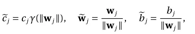
where the vector xinrepresents the signal from all incoming connecting neurons, w are the weights for the input, σ is the activation function, with b as its threshold. In a complex (and deep) network with a large number of neurons, the total number of the free parameters w and b can be exceedingly large. Their training thus poses a tremendous numerical challenge, as the objective function (loss function) to be optimized becomes highly non-convex and with highly complicated landscape [8].Any numerical optimization procedures can be trapped in a local minimum and produce unsatisfactory training results.

This paper is not concerned with numerical algorithm aspect of the NN training. Instead, the purpose of this paper is to show that the training of NNs can be conducted in a reduced parameter space, thus providing any numerical optimization algorithm a smaller space to search for the parameters. This reduction applies to the type of activation functions with the following scaling property: for any α ≥0, σ (α·y)=γ(α)σ(y), where γ depends only on α. The binary activation function [9], one of the first used activation functions, satisfies this property with γ ≡1. The rectified linear unit (ReLU) [10, 11], one of the most widely used activation functions nowadays, satisfies this property with γ =α. For NNs with this type of activation functions, we show that they can be equivalently trained in a reduced parameter space. More specifically, let the length of the weights w be d. Instead of training w in Rd, they can be equivalently trained as unit vector with ∥ w∥=1, which means w ∈Sd?1, the unit sphere in Rd. Moreover, if one is interested in approximating a function defined in a compact domain D, the threshold can also be trained in a bounded interval b ∈[?XB,XB], whereas opposed to the entire real line b ∈R. It is well known that the standard NN with single hidden layer is a universal approximator, cf. Refs. [12–14]. Here we prove that our new formulation in the reduced parameter space is also a universal approximator, in the sense that its span is dense in C (Rd). We then further extend the parameter space constraints to NNs with multiple hidden layers. The major advantage of the constraints in the weights and thresholds is that they significantly reduce the search space for these parameters during training. Consequently, this eliminates a potentially large number of undesirable local minima that may cause training optimization algorithm to terminate prematurely,which is one of the reasons for unsatisfactory training results. We then present examples for function approximation to verify this numerically. Using the same network structure, optimization solver, and identical random initialization, our numerical tests show that the training results in the new reduced parameter space is notably better than those from the standard network.More importantly, the training using the reduced parameter space is much more robust against initialization.

This paper is organized as follows. We first derive the constraints on the parameters using network with single hidden layer, while enforcing the equivalence of the network. Then we prove that the constrained NN formulation remains a universal approximator. After that, we present the constraints for NNs with multiple hidden layers. Finally, we present numerical experiments to demonstrate the improvement of the network training using the reduced parameter space. We emphasize that this paper is not concerned with any particular training algorithm.Therefore, in our numerical tests we used the most standard optimization algorithm from Matlab?. The additional constraints might add complexity to the optimization problem. Efficient optimization algorithms specifically designed for solving these constrained optimization problem will be investigated in a separate paper.

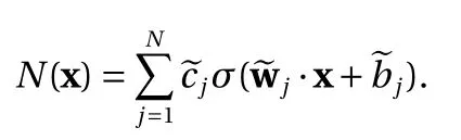
Let us first consider the standard NN with a single hidden layer, in the context for approximating an unknown response function f :Rd→R. The NN approximation using activation function σ takes the following form,

where wj∈Rdis the weight vector, bj∈R the threshold, cj∈R,and N is the width of the network.

We restrict our discussion to following two activation functions. One is the ReLU,

The other one is the binary activation function, also known as heaviside/step function,

with σ (0)=1/2.

We remark that these two activation functions satisfy the following scaling property. For any y ∈R and α ≥0, there exists a constant γ ≥0 such that

where γ depends only on α but not on y. The ReLU satisfies this property with γ (α)=α, which is known as scale invariance. The binary activation function satisfies the scaling property with γ(α)≡1.

We also list the following properties, which are important for the method we present in this paper.

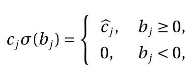
? For the binary activation function Eq. (4), for any x ∈R,

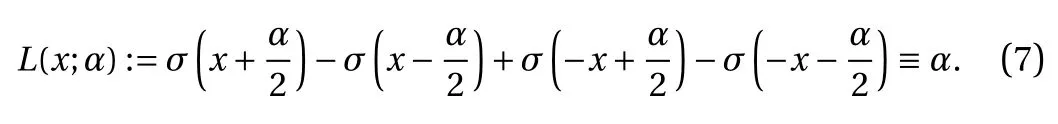
? For the ReLU activation function Eq. (3), for any x ∈R and any α,

We first show that the training of Eq. (2) can be equivalently conducted with constraint ∥ wj∥=1, i.e., unit vector. This is a straightforward result of the scaling property Eq. (5) of the activation function. It effectively reduces the search space for the weights from wj∈Rdto wj∈Sd?1, the unit sphere in Rd.

Proposition 1. Any neural network construction Eq. (2) using the ReLU Eq. (3) or the binary Eq. (4) activation functions has an equivalent form

Proof. Let us first assume ∥ wj∥?=0 for all j =1,2,...,N. We then have

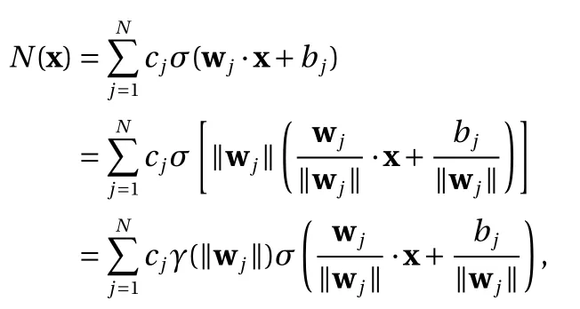
where γ is the factor in the scaling property Eq. (5) satisfied by both ReLU and binary activation functions. Upon defining

we have the following equivalent form as in Eq. (8)

Next, let us consider the case ∥ wj∥=0 for some j ∈{1,2,...,N}.The contribution of this term to the construction Eq. (2) is thus

The proof immediately gives us another equivalent form, by combining all the constant terms from Eq. (2) into a single constant first and then explicitly including it in the expression.

Corollary 2. Any neural network construction Eq. (2) using the ReLU Eq. (3) or the binary Eq. (4) activation functions has an equivalent form

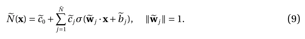
We now present constraints on the thresholds in Eq. (2). This is applicable when the target function f is defined on a compact domain, i.e., f :D →R , with D ?Rdbounded and closed. This is often the case in practice. We demonstrate that any NN Eq. (2)can be trained equivalently in a bounded interval for each of the thresholds. This (significantly) reduces the search space for the thresholds.

Proposition 3. With the ReLU Eq. (3) or the binary Eq. (4) activation function, let Eq. (2) be an approximator to a function f :D →R , where D ?Rdis a bounded domain. Let

Then, Eq. (2) has an equivalent form

Proof. Proposition 1 establishes that Eq. (2) has an equivalent form Eq. (8)

where the bound Eq. (10) is used.

Let us first consider the case

Next, let us consider the case>XB, then·x+>0 for all x ∈D. Let J ={j1,j2,...,jL}, L ≥1, be the set of terms in Eq. (8) that satisfy this condition. We then have·x+>0, for all x ∈D,and ? =1,2,...,L. We now show that the net contribution of these terms in Eq. (8) is included in the equivalent form Eq. (11).

(1) For the binary activation function Eq. (4), the contribution of these terms to the approximation Eq. (8) is

Again, using the relation Eq. (6), any constant can be expressed by a combination of binary activation terms with thresholds=0. Such terms are already included in Eq. (11).

(2) For the ReLU activation Eq. (3), the contribution of these terms to Eq. (8) is

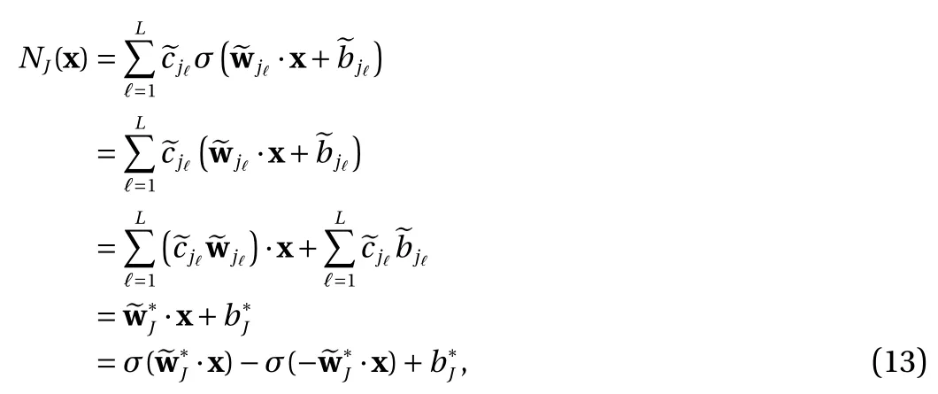
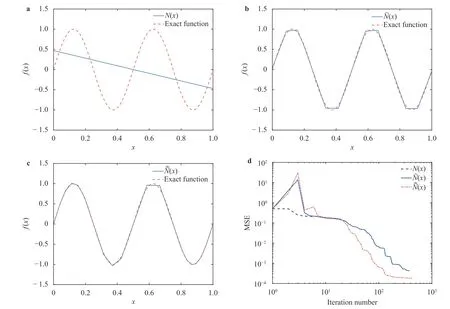
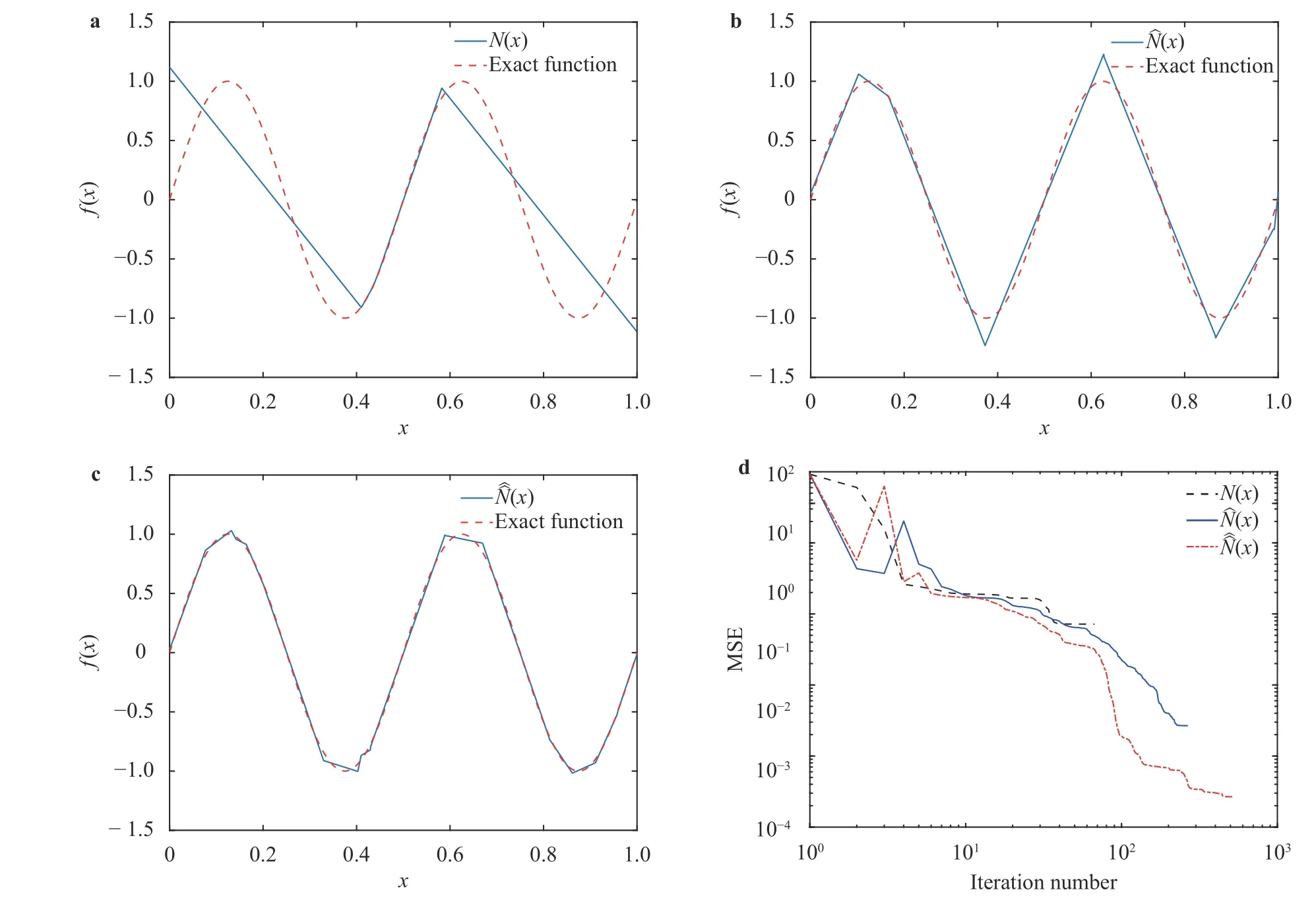
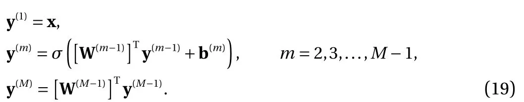
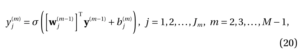
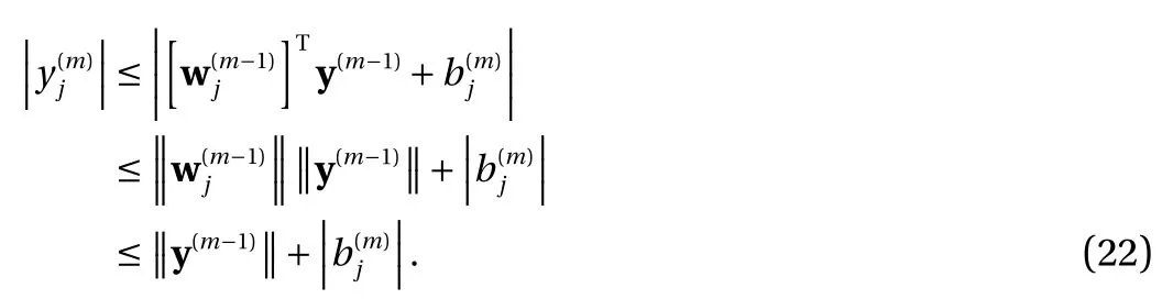
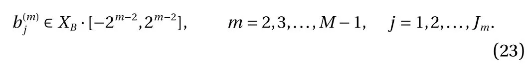
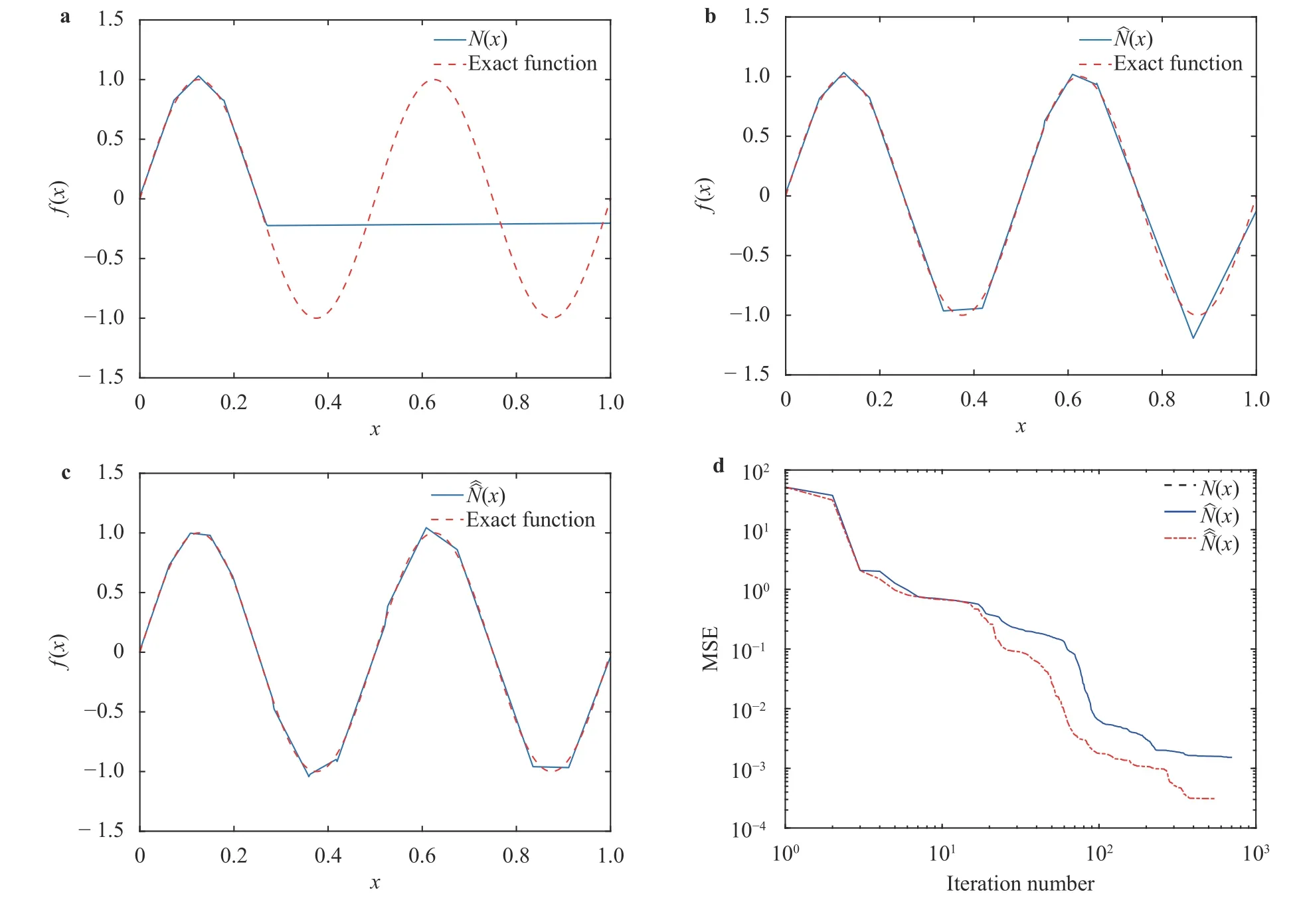
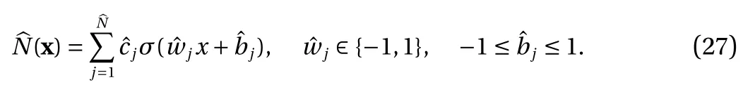
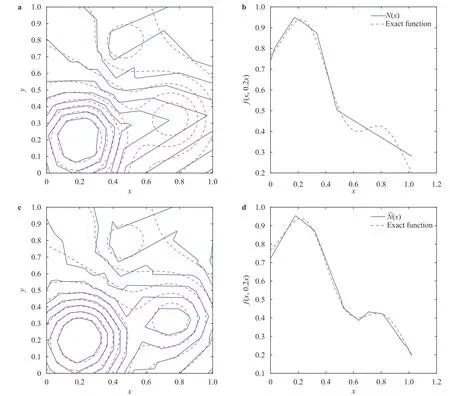
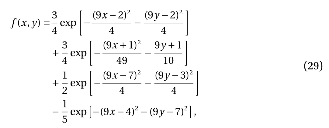
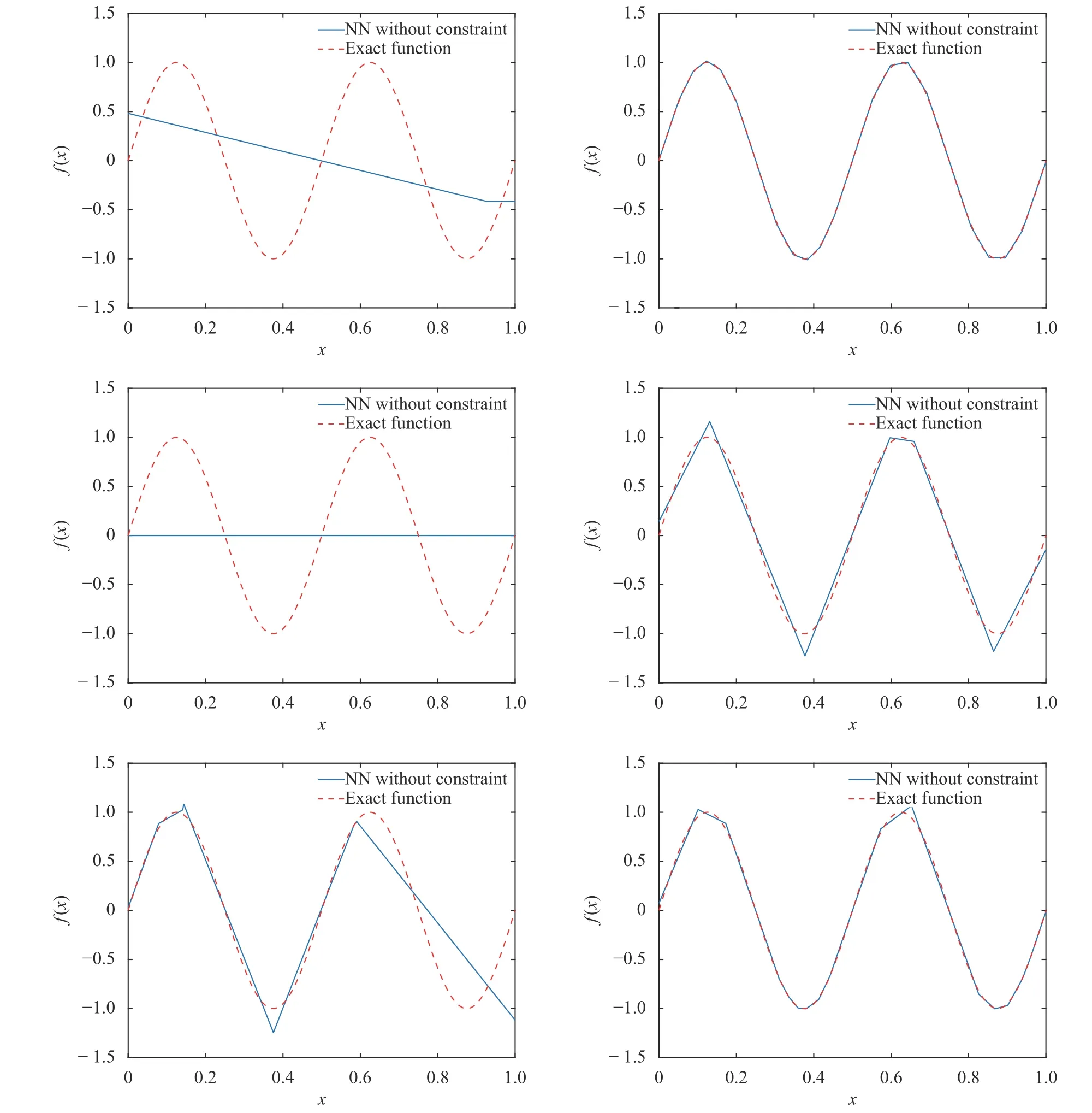
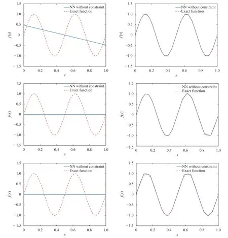
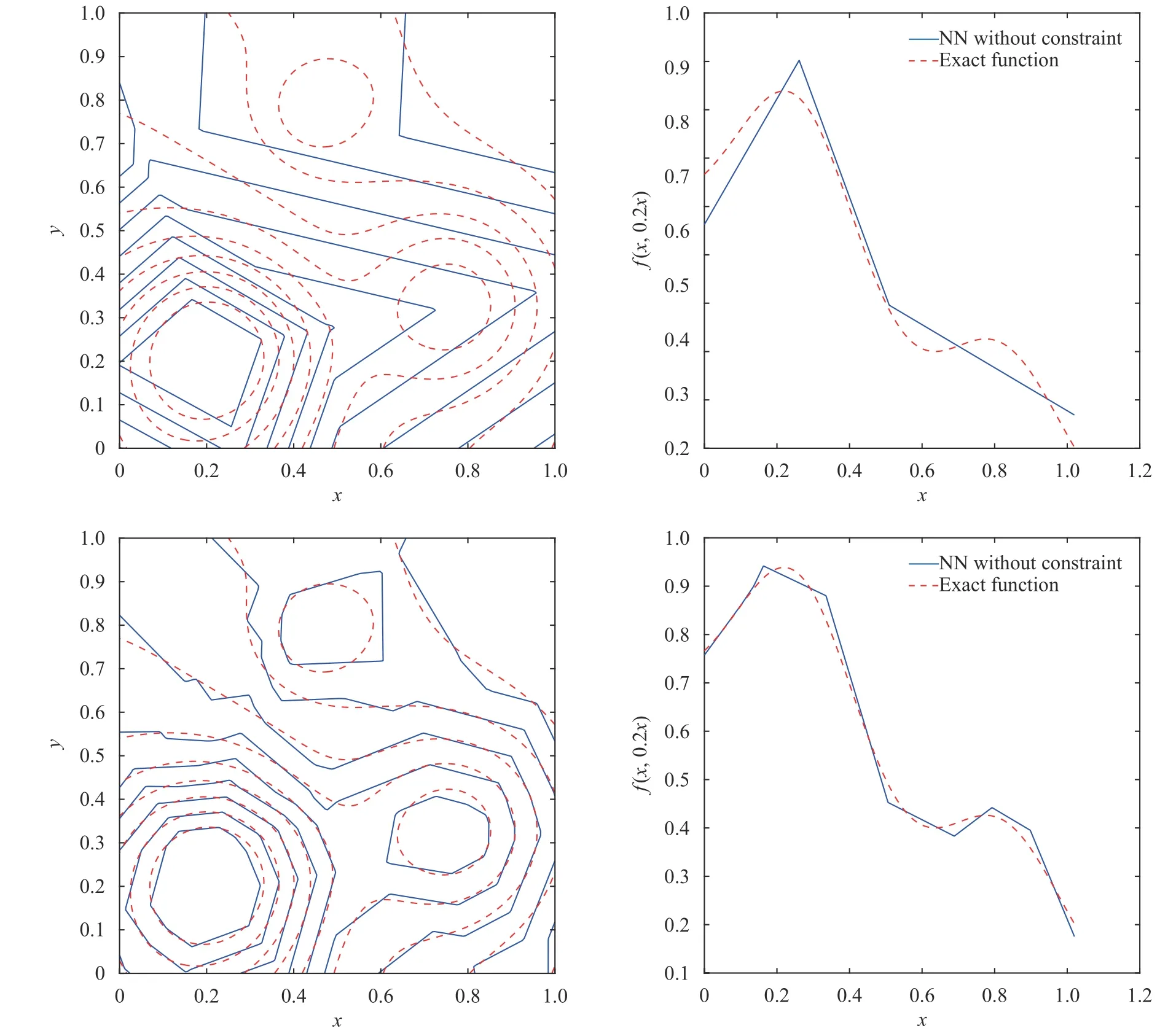
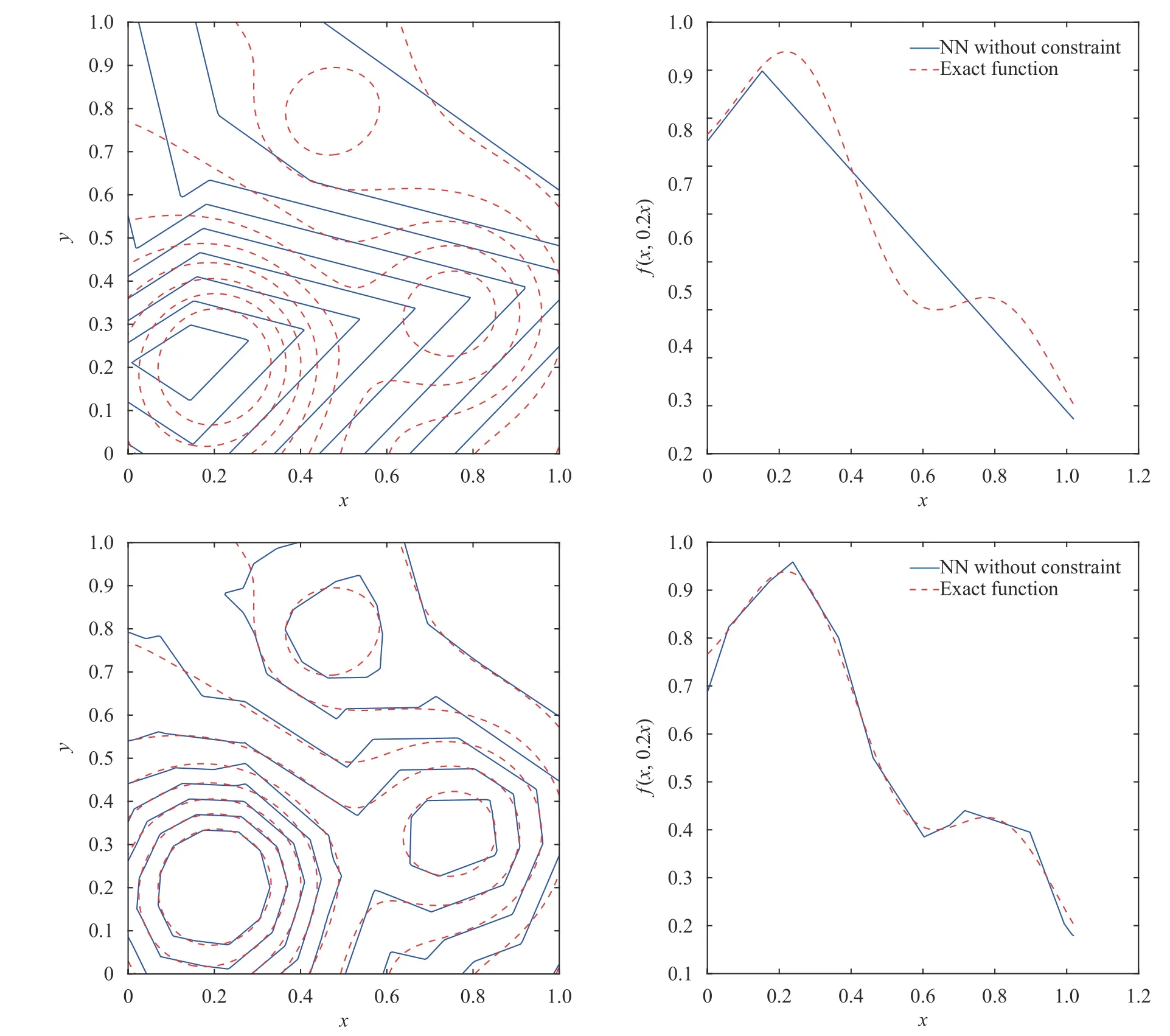
where the last equality follows the simple property of the ReLU function σ(y)?σ(?y)=y. Using Proposition 1, the first two terms then have an equivalent form using unit weightand with zero threshold, which is included in Eq.(11). For the constant, we again invoke the relation Eq. (7) and represent it bywhereis an arbitrary unit vector and 0 <α

We remark that the equivalent form in the reduced parameter space Eq. (11) has different number of “active” neurons than the original unrestricted case Eq. (2). The equivalence between the standard NN expression Eq. (2) and the constrained expression Eq. (11) indicates that the NN training can be conducted in a reduced parameter space. For the weights wjin each neuron,its training can be conducted in Sd?1, the d-dimensional unit sphere, as opposed to the entire space Rd. For the threshold, its training can be conducted in the bounded interval [? XB,XB], as opposed to the entire real line R. The reduction of the parameter space can eliminate many potential local minima and therefore enhance the performance of numerical optimization during the training.

This advantage can be illustrated by the following one dimensional example. Consider an NN with one neuron N(x)=cσ(wx+b). Suppose we are given one data point ( 1,1),then we would like to fix parameters c ∈R, w ∈R and b ∈R by minimizing the following mean squared loss, i.e.,

Global minimizers for this objective function lie in the set

By the definition of the ReLU function, in the region

we have J (c,w,b)≡1, which means every point in Z is a local minima.

However, if we consider the equivalent minimization problem in the reduced parameter space, i.e.,

The local minima set now is reduced to

which is much smaller than Z.

By universal approximation property, we aim to establish that the constrained formulations Eqs. (8) and (11) can approximate any continuous function. To this end, we define the following set of functions on Rd

where Λ ∈Rdis the weight set, Θ ∈R the threshold set. We also denote ND(σ;Λ,Θ) as the same set of functions when confined in a compact domain D ?Rd.

By following this definition, the standard NN expression and our two constrained expressions correspond to the following spaces

where Sd?1is the unit sphere in Rdbecause=1.

The universal approximation property for the standard unconstrained NN expression Eq. (2) has been well studied, cf.Refs. [13-17], and Ref. [12] for a survey. Here we cite the following result for N (σ;Rd,R).

Theorem 4 (Ref. [17], Theorem 1). Let σ be a function in(R), of which the set of discontinuities has Lebesgue measure zero. Then the set N (σ;Rd,R) is dense in C (Rd), in the topology of uniform convergence on compact sets, if and only if σ is not an algebraic polynomial almost everywhere.

We now examine the universal approximation property for the first constrained formulation Eq. (8).

Theorem 5. Let σ be the binary function Eq. (4) or the ReLU function Eq. (3), then we have

and the set N (σ;Sd?1,R) is dense in C (Rd), in the topology of uniform convergence on compact sets.

Proof. Obviously, we have N (σ;Sd?1,R)?N(σ;Rd,R). By Proposition 1, any element N (x)∈N(σ;Rd,R) can be reformulated as an element N (x)∈N(σ;Sd?1,R). Therefore, we have N(σ;Rd,R)?N(σ;Sd?1,R). This concludes the first statement Eq. (17). Given the equivalence Eq. (17), the denseness result immediately follows from Theorem 4, as both the ReLU and the binary activation functions are not polynomials and are continuous everywhere except at a set of zero Lebesgue measure.

We now examine the second constrained NN expression Eq.(11).

Fig. 1. Numerical results for Eq. (26) with one sequence of random initialization.

Theorem 6. Let σ be the binary Eq. (4) or the ReLU Eq. (3) activation function. Let x ∈D ?Rd, where D is closed and bounded with. Define Θ =[?XB,XB], then

Furthermore, ND(σ;Sd?1,Θ) is dense in C (D) in the topology of uniform convergence.

Proof. Obviously we have ND(σ;Sd?1,Θ)?ND(σ;Rd,R). On the other hand, Proposition 3 establishes that for any element N(x)∈ND(σ;Rd,R), there exists an equivalent formulation(x)∈ND(σ;Sd?1,Θ) for any x ∈D. This implies ND(σ;Rd,R)?ND(σ;Sd?1,Θ). We then have Eq. (18).

For the denseness of ND(σ;Sd?1,Θ) in C (D), let us consider any function f ∈C(D). By the Tietze extension theorem (cf. Ref.[18]), there exists an extension F ∈C(Rd) with F (x)=f(x) for any x ∈D. Then, the denseness result of the standard unconstrained E={x ∈Rd:∥x∥≤XB} and any given ?>0, there exists N(x)∈N(σ;Rd,R) such that NN expression (Theorem 4) implies that, for the compact set

By Proposition 3, there exists an equivalent constrained NN expression∈ND(σ;Sd?1,Θ) such that N(x)=N(x) for any x ∈D. We then immediately have, for any f ∈C(D) and any given ?>0, there exists N (x)∈ND(σ;Sd?1,Θ) such that

Fig. 2. Numerical results for Eq. (26) with a second sequence of random initialization.

The proof is now complete.

We now generalize the previous result to feedforward NNs with multiple hidden layers. Let us again consider approximation of a multivariate function f :D →R , where D ?Rdis a compact subset of Rdwith

Consider a feedforward NN with M layers, M ≥3, where m=1 is the input layer and m =M the output layer. Let Jm,m=1,2,...,M be the number of neurons in each layer. Obviously, we have J1=d and JM=1 in our case. Let y(m)∈RJmbe the output of the neurons in the m-th layer. Then, by following the notation from Ref. [5], we can write

where W(m?1)∈RJm?1×Jmis the weight matrix and b(m)is the threshold vector. In component form, the output of the j-th neuron in the m-th layer is

The derivation for the constraints on the weights vectorcan be generalized directly from the single-layer case and we have the following weight constraints,

The constraints on the thresholddepend on the bounds of the output from the previous layer y(m?1).

For the ReLU activation function Eq. (3), we derive from Eq.(20) that for m =2,3,...,M,

If the domain D is bounded and withthen the constraints on the threshold can be recursively derived.Starting from ∥ y(1)∥=∥x∥∈[?XB,XB] and b(j2)∈[?XB,XB], we then have

For the binary activation function Eq. (4), we derive from Eq.(20) that for m =2,3,...,M ?1,

Then, the bounds for the thresholds are

We present numerical examples to demonstrate the properties of the constrained NN training. We focus exclusively on the ReLU activation function Eq. (3) due to its overwhelming popularity in practice.

Given a set of training samples, the weights and thresholds are trained by minimizing the following mean squared error (MSE)

We conduct the training using the standard unconstrained NN formulation Eq. (2) and our new constrained Eq. (11) and compare the training results. In all tests, both formulations use exactly the same randomized initial conditions for the weights and thresholds. Since our new constrained formulation is irrespective of the numerical optimization algorithm, we use one of the most accessible optimization routines from MATLAB?, the function fminunc for unconstrained optimization and the function fmincon for constrained optimization. For the optimization options, we use the sequential quadratic programming (spg) algorithm for both the constrained and unconstrained optimization, with the same optimality tolerance 10?6and maximum iteration number 1500. It is natural to explore the specific form of the constraints in Eq. (11) to design more effective constrained optimization algorithms. This is,however, out of the scope of the current paper.

Fig. 3. Numerical results for Eq. (26) with a third sequence of random initialization

After training the networks, we evaluate the network approximation errors using another set of samples—a validation sample set, which consists of randomly generated points that are independent of the training sample set. Even though our discussion applies to functions in arbitrary dimension d ≥1, we present only the numerical results in d =1 and d =2 because they can be easily visualized.

We first examine the approximation results using NNs with single hidden layer, with and without constraints.

We first consider a one-dimensional smooth function

The constrained formulation Eq. (11) becomes

Due to the simple form of the weights and the domain D =[0,1],the proof of Proposition 3 also gives us the following tighter bounds for the thresholds for this specific problem,

Fig. 4. Numerical results for Eq. (29). a Unconstrained formulation N (x) in Eq. (2). b Constrained formulation N (x) in Eq. (11).

We approximate Eq. (26) with NNs with one hidden layer,which consists of 2 0 neurons. The size of the training data set is 200. Numerical tests were performed for different choices of random initializations. It is known that NN training performance depends on the initialization. In Figs. 1–3, we show the numerical results for three sets of different random initializations. In each set, the unconstrained NN Eq. (2), the constrained NN Eq.(27) and the specialized constrained NN with Eq. (28) use the same random sequence for initialization. We observe that the standard NN formulation without constraints (2) produces training results critically dependent on the initialization. This is widely acknowledged in the literature. On the other hand, our new constrained NN formulations are more robust and produce better results that are less sensitive to the initialization. The tighter constraint Eq. (28) performs better than the general constraint Eq. (27), which is not surprising. However, the tighter constraint is a special case for this particular problem and not available in the general case.

We next consider two-dimensional functions. In particular,we show result for the Franke's function [19]

Fig. 5. Numerical results for 1D function Eq. (26) with feedforward NNs of { 1,20,10,1}. From top to bottom: training results using three different random sequences for initialization. Left column: results by unconstrained NN formulation Eq. (19). Right column: results by NN formulation with constraints Eqs. (21) and (23).

with ( x,y)∈[0,1]2. Again, we compare training results for both the standard NN without constraints Eq. (2) and our new constrained NN Eq. (8), using the same random sequence for initialization. The NNs have one hidden layer with 4 0 neurons.The size of the training set is 5 00 and that of the validation set is 1000. The numerical results are shown in Fig. 4. On the left column, the contour lines of the training results are shown, as well as those of the exact function. Here all contour lines are at the same values, from 0 to 1 with an increment of 0.1. We observe that the constrained NN formulation produces visually better result than the standard unconstrained formulation. On the right column, we plot the function value along y=0.2x.Again, the improvement of the constrained NN is visible.

We now consider feedforward NNs with multiple hidden layers. We present results for both the standard NN without constraints Eq. (19) and the constrained ReLU NNs with the constraints Eqs. (21) and (23). We use the standard notation{J1,J2,...,JM} to denote the network structure, where Jmis the number of neurons in each layer. The hidden layers are J2,J3,...,JM?1. Again, we focus on 1D and 2D functions for ease of visualization purpose, i.e., J1=1,2.

Fig. 6. Numerical results for 1D function Eq. (26) with feedforward NNs of { 1,10,10,10,10,1}. From top to bottom: training results using three different random sequences for initialization. Left column: results by unconstrained NN formulation Eq. (19). Right column: results by NN formulation with constraints Eqs. (21) and (23).

We first consider the one-dimensional function Eq. (26). In Fig. 5, we show the numerical results by NNs of { 1,20,10,1}, using three different sequences of random initializations, with and without constraints. We observe that the standard NN formulation without constraints Eq. (19) produces widely different results. This is because of the potentially large number of local minima in the cost function and is not entirely surprising. On the other hand, using the exactly the same initialization, the NN formulation with constraints Eqs. (21) and (23) produces notably better results, and more importantly, is much less sensitive to the initialization. In Fig. 6, we show the results for NNs with{1,10,10,10,10,1} structure. We observe similar performance—the constrained NN produces better results and is less sensitive to initialization.

We now consider the two-dimensional Franke's function Eq.(29). In Fig. 7, the results by NNs with { 2,20,10,1} structure are shown. In Fig. 8, the results by NNs with { 2,10,10,10,10,1} structure are shown. Both the contour lines (with exactly the same contour values: from 0 to 1 with increment 0.1) and the function value at y =0.2x are plotted, for both the unconstrained NN Eq.(19) and the constrained NN with the constraints Eqs. (21) and(23). Once again, the two cases use the same random sequence for initialization. The results show again the notably improvement of the training results by the constrained formulation.

In this paper we presented a set of constraints on multi-layer feedforward NNs with ReLU and binary activation functions. The weights in each neuron are constrained on the unit sphere, as opposed to the entire space. This effectively reduces the number of parameters in weights by one per neuron. The threshold in each neuron is constrained to a bounded interval, as opposed to the entire real line. We prove that the constrained NN formulation is equivalent to the standard unconstrained NN formulation. The constraints on the parameters, even though may increase the complexity of the optimization problem, reduce the search space for network training and can potentially improve the training results. Our numerical examples for both single hidden layer and multiple hidden layers verify this finding.

Fig. 7. Numerical results 2D function Eq. (29) with NNs of the structure { 2,20,10,1}. Top row: results by unconstrained NN formulation Eq.(19). Bottom row: results by constrained NN with Eqs. (21) and (23). Left column: contour plots. Right column: function cut along y =0.2x.Dashed lines are the exact function.

Fig. 8. Numerical results 2D function Eq. (29) with NNs of the structure { 2,10,10,10,10,1}. Top row: results by unconstrained NN formulation Eq. (19). Bottom row: results by constrained NN with Eqs. (21) and (23). Left column: contour plots. Right column: function cut along y =0.2x.Dashed lines are the exact function.