THE QUASI-BOUNDARY VALUE METHOD FOR IDENTIFYING THE INITIAL VALUE OF THE SPACE-TIME FRACTIONAL DIFFUSION EQUATION ?
2020-08-03 07:13:48FanYANG楊帆YanZHANG張燕XiaoLIU劉霄XiaoxiaoLI李曉曉
Fan YANG ( 楊帆 ) Yan ZHANG (張燕) Xiao LIU (劉霄) Xiaoxiao LI (李曉曉)
Department of Mathematics, Lanzhou University of Technology, Lanzhou 730050, China E-mail: yfggd114@163.com; yanzhanglut@163.com; liuxiaolut@163.com; lixiaoxiaogood@126.com
Abstract In this article, we consider to solve the inverse initial value problem for an in-homogeneous space-time fractional diffusion equation. This problem is ill-posed and thequasi-boundary value method is proposed to deal with this inverse problem and obtain the series expression of the regularized solution for the inverse initial value problem. We prove the error estimates between the regularization solution and the exact solution by using an a pri-ori regularization parameter and an a posteriori regularization parameter choice rule. Some numerical results in one-dimensional case and two-dimensional case show that our method is efficient and stable.
Key words Space-time fractional diffusion equation; Ill-posed problem; quasi-boundary value method; identifying the initial value
1 Introduction
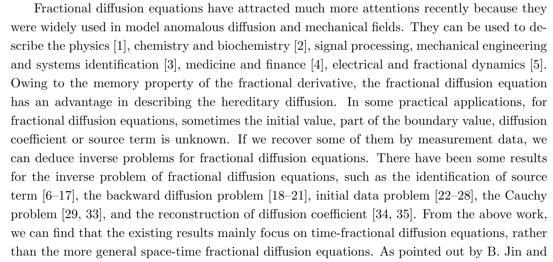
W. Rundell’s article [36], the study of space-fractional inverse problem, either theoretical or numerical, is quite scarce. In [37], the authors proved the uniqueness of the inverse source problem for a space-time fractional equation. In [38], the authors applied Fourier truncation method to solve an inverse source problem for space-time fractional equation.
In this article, we consider the following inhomogeneous space-time fractional diffusion equation:

where ? := (?1,1), r > 0 is a parameter, F(x,t) ∈L∞[0,T;L2(?)], g(x) ∈L2(?) are given function, β ∈(0,1) and α ∈(1,2) are fractional order of the time and the space derivatives,respectively, and T > 0 is a final time. The time-fractional derivativeis the Caputo fractional derivative with respect to t of the order β defined by

in which Γ(x) is the standard Gamma function.
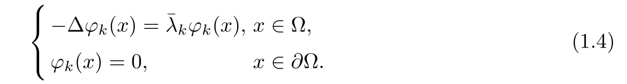
Note that if the fractional order β tends to unity, the fractional derivativeconverges to the first-order derivative[5], and thus the problem reproduces the diffusion model; see,for example,[5,39]for the definition and properties of Caputo’s derivative. We introduce a few properties of the eigenvalues of the operator ??(see [39, 40]). Denote the eigenvalues of ??as, and suppose thatsatisfy

and the corresponding eigenfunctions ?k(x). Therefore, (,?k(x)), k =1,2,···, satisfy
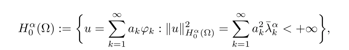
Define

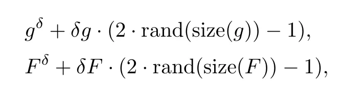
In problem (1.1), the source function F(x,t) and the final value data g(x) are given. We reconstruct the initial function u(x,0)=f(x)∈L2(?) from noisy data (gδ,Fδ) which satisfies

where the constant δ >0 represents the noise level.
In this study, we main exploit the quasi-boundary value regularization method to identify the initial value of a space-time fractional diffusion equation by two measurable data. The quasi-boundary value regularization method is a very effective method for solving ill-posed problems and has been discussed to solve different types of inverse problems [41–45].
This article is organized as follows. We introduce some preliminaries results in Section 2. In Section 3, we analyze the ill-posedness of this problem and give a conditional stability results. In Section 4, we exploit the quasi-boundary value regularization method and present the error estimates under an a priori regularization parameter selection rule and an a posteriori regularization parameter selection rule,respectively. In Section 5,some numerical results in the one-dimensional case and two-dimensional case show that our method is efficient and stable.We give a simple conclusion in Section 6.
2 Preliminary Results
Now, we introduce some useful definitions and preliminary results.
Definition 2.1([46]) The Mittag-leffler function is

where α>0 and β ∈R are arbitrary constants.
Lemma 2.2([46]) Let λ>0 and 0<β <1, then we have

Lemma 2.3([46]) Let λ>0, then

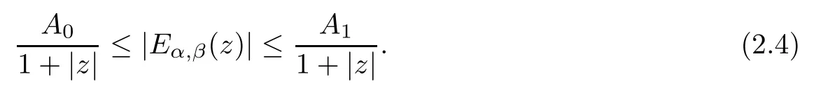
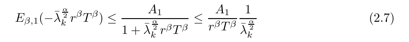
Lemma 2.4([37]) If α ≤2, β is arbitrary real number,< μ < min{πα,π}, μ ≤|arg(z)|≤π, then there exists two constant A0>0 and A1>0, such that
Lemma 2.5([8]) Let Eβ,β(?η)≥0, 0<β <1, we have

Lemma 2.6Forsatisfying>0, there exists positive constants C1,C2which depend on β,T,, such that

ProofBy Lemma 2.4, we have
and

The proof of Lemma is completed.
3 Problem Analysis
The exact solution u of direct problem (1.1) is given in form [37, 47]
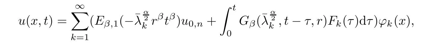

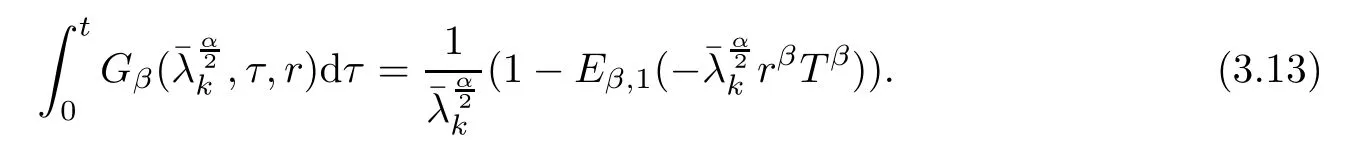
where fk=(f(x),?k(x)), Fk=(F(x,t),?k(x)), and Gβ(,t,r) is denoted by

Using u(x,T)=g(x), we obtain

According to Fourier series expansion, g(x) can also be rewritten as. Thus,

Hence,
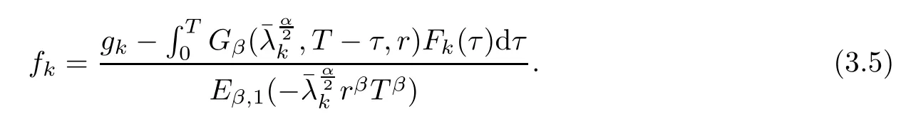

Thus,
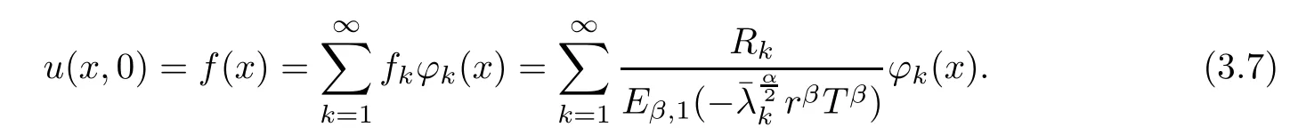
In order to find f(x), we need to solve the following integral equation

where the kernel is
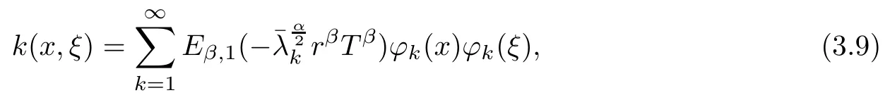
where k(x,ξ) = k(ξ,x), so K is self adjoint operator. From [8], we know that K : L2(?) →L2(?) is a compact operator, so problem (1.1) is ill-posed. Suppose that f(x) has a priori bound as follows:

where E >0 is a constant.
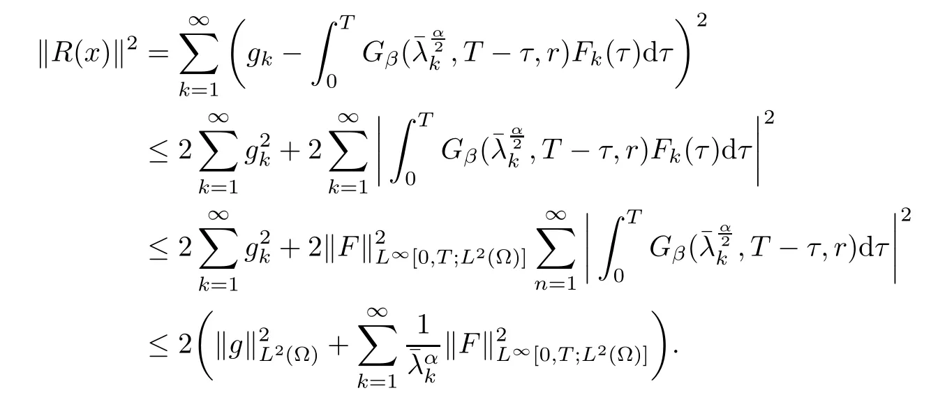
Lemma 3.1Let F ∈L∞[0,T;L2(?)] and R(x) be given by (3.6). Then, there exists a positive M such that

ProofFor 0 ≤t ≤T, there holds

Using Lemma 2.2 and Eα,1(0)=1 lead to
Using Lemma 2.5, we get

so
Hence, the proof is completed.
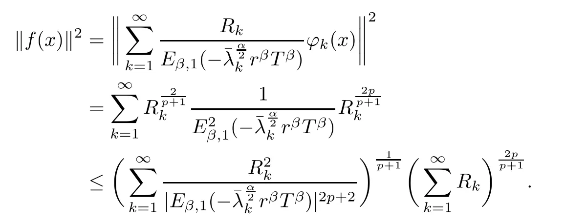
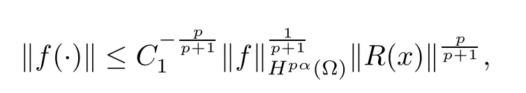
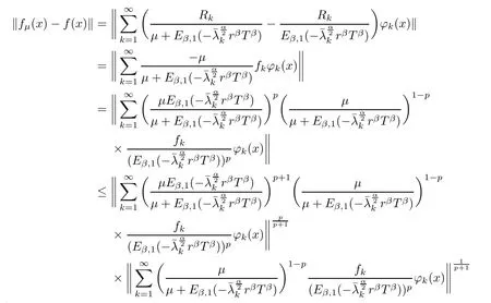
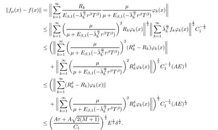
Theorem 3.2(A conditional stability estimate) Assume that there exist p>0 such that≤E. Then,

ProofUsing (3.7) and H?lder inequality, we have
Using Lemma 2.6, we get
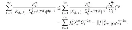
So,
4 The Quasi-Boundary Value Regularization Method and Error Estimates
In this section, the quasi-boundary value regularization method is proposed to solve the problem (1.1) and give the error estimate under the priori parameter selection rule and the posteriori parameter selection rule, respectively.
In nature, we will investigate the following problem:
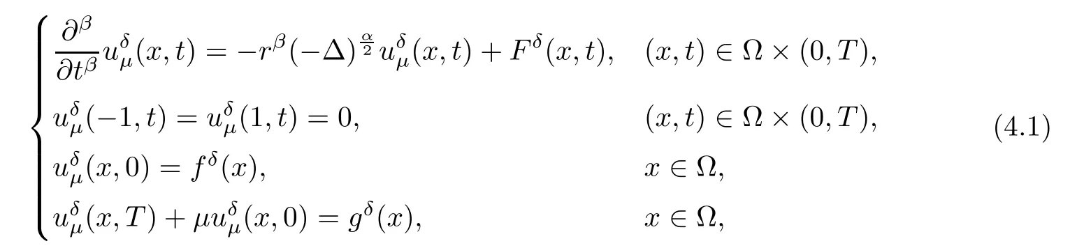
where μ > 0 is a regularized parameter. This method is called quasi-boundary value regularization method.
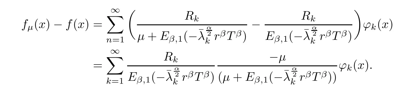
Using the separation of variable, we can obtain


So,

4.1 Error estimate under an a priori parameters choice rule
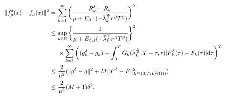
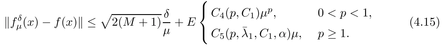
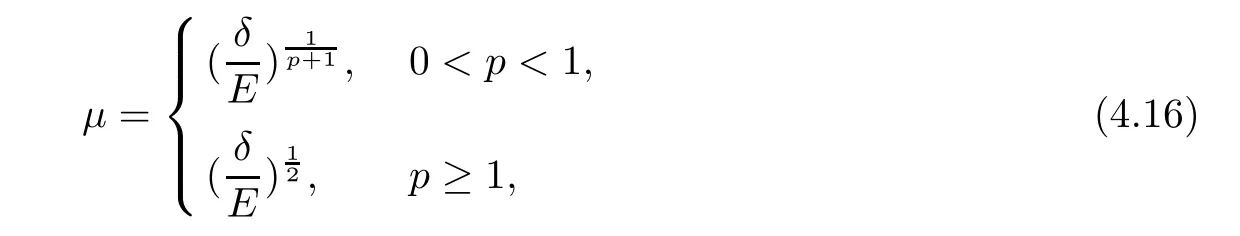
Theorem 4.1Let f(x) given by (3.7) be the exact solution of problem (1.1). Letgiven by (4.4) be the regularization solution. Suppose that the a priori condition (3.10) and(1.6) hold, we can obtain the following results:
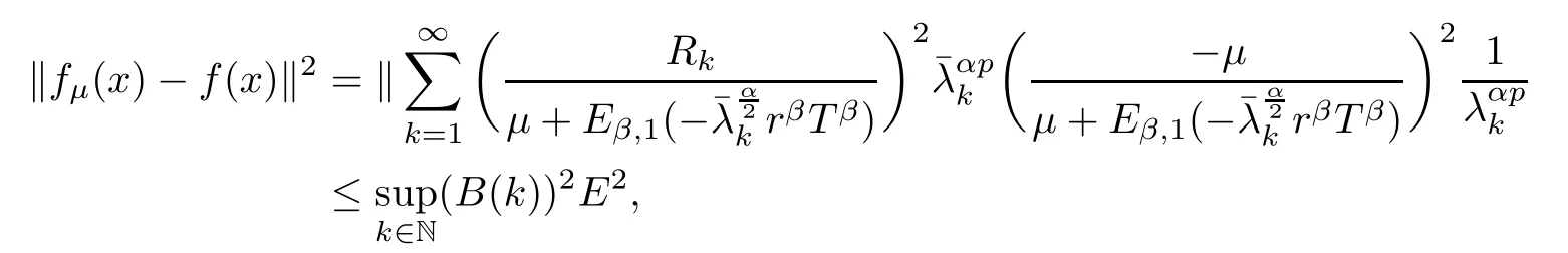
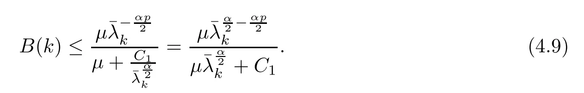
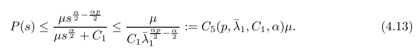
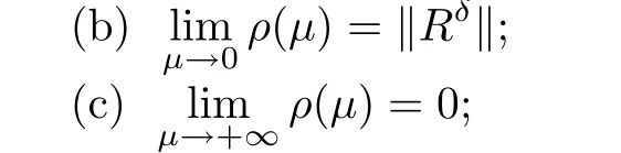
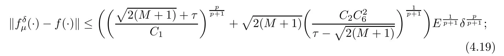
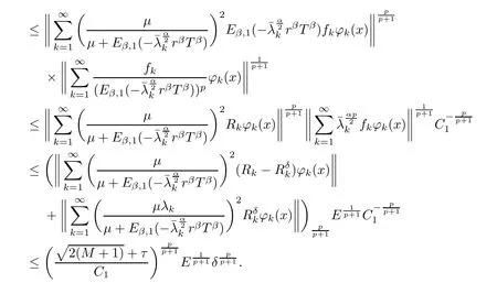
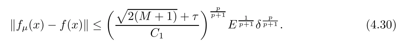
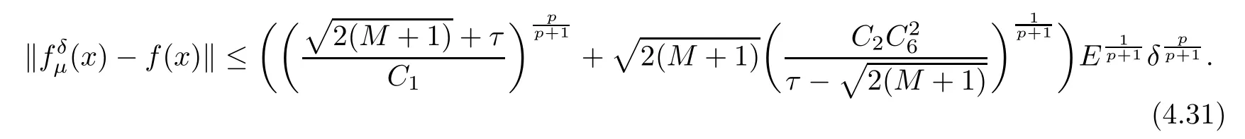
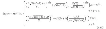
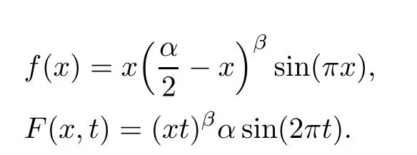
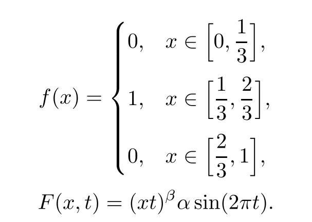
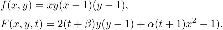
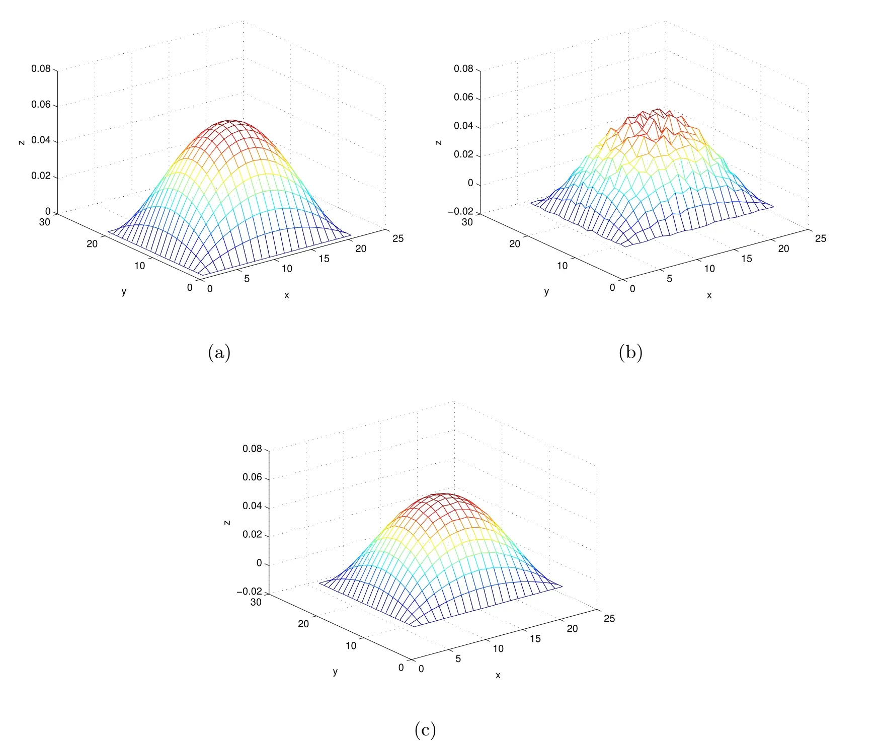
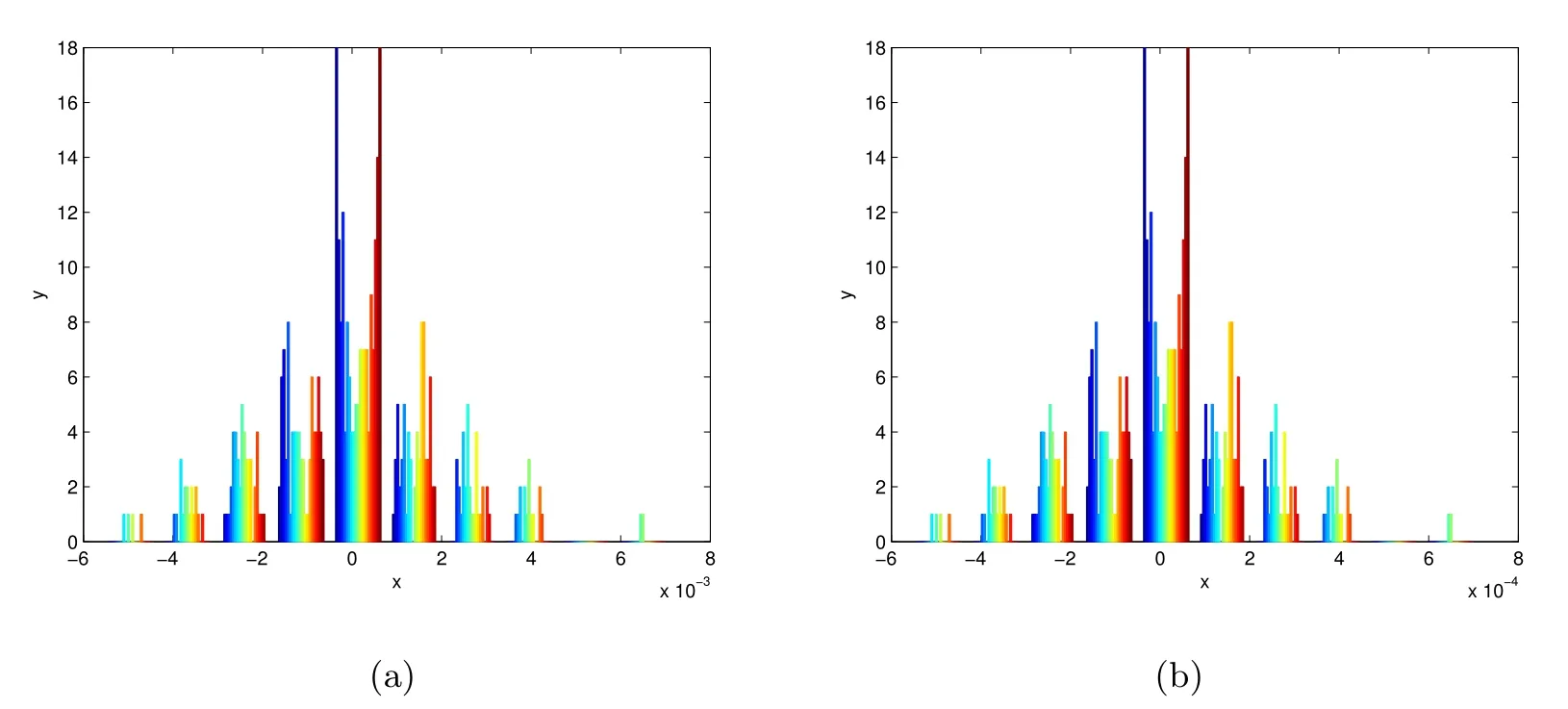
(1) If 0 where C4=C4(p,C1)>0, C5=C5(p,,C1,α)>0. ProofApplying (3.7), (4.4), and triangle inequality, we have We first estimate the first term of (4.7). Using (1.6) and Lemma 3.1, we obtain Hence, Next, we estimate second items of (4.7). By (4.4), we have Applying the priori bound condition (3.10), we get Using Lemma 2.6, we obtain Suppose that s0is the root of P′(s0)=0, then we get If 0 If p ≥1, we have Hence, So, Choosing the regularization parameter μ as follows: we obtain We apply a discrepancy principle in the following form: Lemma 4.2Letif, then we have the following conclusions: (a) ρ(μ) is a continuous function; (d) ρ(μ) is a strictly decreasing function, for any μ∈(0,+∞). Theorem 4.3Let f(x) given by (3.7) be the exact solution of problem (1.1). Letgiven by(4.4)be the regularization solution. The regularization parameterμis chosen in(4.18).Then, we have the following results: (1) If 0 (2) If p ≥1, we obtain the error estimate: ProofUsing the triangle inequality, we obtain We first estimate the first term of (4.21). By (4.18) and Lemma 2.6, we have Suppose that s?is the root of T′(s?)=0, then we get If 0 If p ≥1, we have Hence, Choose the regularization parameter μ as follows: For 0 Now, we estimate the second term of (4.21). Using (1.6), Lemma 2.6, and H?lder inequality,we have Hence, Combining (4.28) and (4.30), we obtain (2) If p ≥1, Hαp(?) compacts into Hα(?), then there exists a positive number such thatHence, So, Therefore, we obtain Hence, the proof of Theorem 4.3 is completed. In this section, several different examples are described to verify our present regularization method. Because the analytic solution of problem (1.1) is hard to receive, we solve the forward problem with the given data f(x) and F(x,t) by a finite difference method to construct the final data u(x,T)=g(x). The noisy data is generated by adding a random perturbation, that is, the magnitude δ indicates a relative noise level. For simplicity, we assume that the maximum time is T = 1. In order to compute Mittag-Leffler function, we need a better algorithm [48]. Because the a priori bound E is difficult to obtain, we only give the numerical results by using the a posteriori parameter choice rule. The regularization parameter is given by (4.18) with τ = 1.1. Here, we use the dichotomy method to find μ. Example 1Choose Example 2Choose In Figure 1,we show the comparisons between the exact solution and its regularized solution for various noise levels δ =0.0001,0.00005,0.00001 in the case of β =0.2,0.7,α=1.9. In Figure 2, we show the comparisons between the exact solution and its regularized solution for various noise levels δ = 0.0001,0.00005,0.00001 in the case of β = 0.2,0.7, α = 1.7. The numerical results become less accurate as the fractional orders α and the noise level increase. Figure 1 The comparison of the numerical effects between the exact solution and its computed approximations. (a) β =0.2, α=1.9. (b) β =0.7, α=1.9 Figure 2 The comparison of the numerical effects between the exact solution and its computed approximations. (a) β =0.2, α=1.7. (b) β =0.7, α=1.7 In Figure 3,we show the comparisons between the exact solution and its regularized solution for various noise levels δ =0.0001,0.00005,0.00001 in the case of β =0.2,0.7,α=1.9. In Figure 4, we show the comparisons between the exact solution and its regularized solution for various noise levels δ =0.0001,0.00005,0.00001 in the case of β =0.2,0.7,α=1.7. It can be seen that our proposed method is also effective for solving the discontinuous example. Figure 3 The comparison of the numerical effects between the exact solution and its computed approximations. (a) β =0.2, α=1.9. (b) β =0.7, α=1.9 Figure 4 The comparison of the numerical effects between the exact solution and its computed approximations. (a) β =0.2, α=1.7. (b) β =0.7, α=1.7 Example 3Choose In Figure 5, 7,we show the comparisons between the exact solution and its regularized solution for various noise levels δ = 0.00001,0.000001. In Figure 6, we show the error of the exact solution and its regularized solution. It can be seen that the proposed method is also valid for solving the two-dimensional example. Figure 5 The comparison of the numerical effects between the exact solution and its computed approximations. (a) The exact solution. (b) ε=0.00001. (c) ε=0.000001 Figure 6 (a) Numerical error for ε=0.00001. (b) Numerical error for ε=0.000001 Figure 7 The comparison of the numerical effects between the exact solution and its computed approximations. (a) The exact solution. (b) ε=0.00001. (c) ε=0.000001 In this article, we investigate the inverse initial value problem of an inhomogeneous spacetime fractional diffusion equation. The conditional stability is given. The quasi-boundary value regularization method is proposed to obtain a regularization solution. The error estimates are obtained under an a priori regularization parameter choice rule and an a posteriori regularization parameter choice rule, respectively. Finally, some numerical results show the utility of the used regularization method. In the future work, we will continue to research the inverse problems of fractional equations in identifying the source term and the initial value.


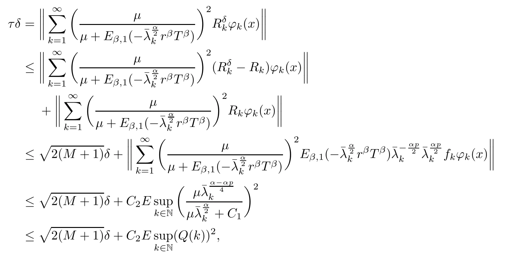
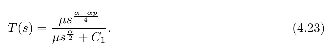
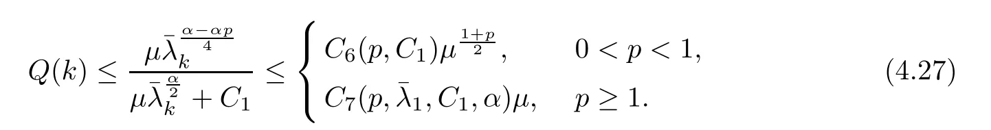
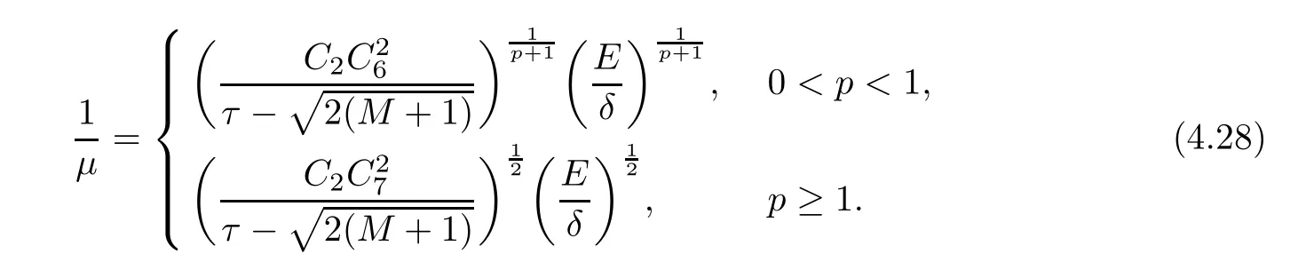
4.2 An a posteriori regularization parameter choice rule and Error estimate


5 Numerical Experiments
5.1 One-dimensional case


5.2 Two-dimensional case

6 Conclusion
 Acta Mathematica Scientia(English Series)2020年3期