Exact explicit solitary wave and periodic wave solutions and their dynamical behaviors for the Schamel–Korteweg–de Vries equation?
2021-06-26 03:31:08BinHe何斌andQingMeng蒙清
Chinese Physics B 2021年6期
Bin He(何斌) and Qing Meng(蒙清)
College of Mathematics and Statistics,Honghe University,Mengzi 661100,China
Keywords: Schamel–Korteweg–de Vries equation,dynamical behavior,solitary wave solution,periodic wave
1. Introduction
The Schamel–Korteweg–de Vries (Schamel-KdV)equation[1–18]can be written as

whereα,βandδare constants anduis the wave potential,which arises in the study of ion acoustic solitons in plasma physics when electron trapping is present, and also it governs the electrostatic potential for a certain electron distribution in velocity space.[1,2]We mention that Eq.(1)reduces to the well-known KdV equation[3,4]whenα=0 and reduces to the Schamel equation[5–7]whenβ=0. It is known that the KdV equation has other kinds of explicit solutions,particularly rational solutions,[8]which provide better approximations to real physical nonlinear waves in terms of the complexity and computational time. More generally, lump solutions could exist in the Kadomtsev–Petviashvili equation[9]and other(2+1)-generalizations of the KdV equation.[10]Due to the wide range of applications of Eq.(1),it is important to find its new exact wave solutions.Khateret al.[11]obtained the periodic wave solutions using the F-expansion method. Lee and Sakthivel[12]proposed the Exp-function method to generate a rich class of traveling wave solutions. Using a extended mapping method and the availability of symbolic computation, several classes of exact solutions are expressed by various JEFs and hyperbolic functions.[13]Wu and Liu[14]found two types of nonlinear wave solutions called compacton-like wave and kink-like wave solutions. The hyperbolic function solutions and the trigonometric function solutions with free parameters have been obtained in Ref. [15] using theG'/Gexpansion method. Giresunluet al.[16]obtained exact traveling wave solutions using Lie symmetry analysis together with the simplest equation method and the Kudryashov method,and constructed exact solutions using the conservation laws and symmetries of the underlying equation. Some analytical solutions are given in Ref.[17]using direct integration for negative and positive phase velocities. Applying the direct method and the method of elliptic ordinary differential equations,Kengneet al.[18]found some exact solutions and so forth.
There are some interesting problems: How do solitary wave and periodic wave solutions depend on parameters of a system? Are there dynamical behaviors of solitary wave and periodic wave solutions to Eq. (1)? To our knowledge, these problems have not been considered before for Eq.(1). In this paper, we consider the existence and dynamical behaviors of the exact explicit solitary wave and periodic wave solutions to Eq. (1) in different regions of the parametric space. We also give all possible exact explicit parametric representations for solitary wave and periodic wave solutions to Eq.(1). The present results more completely answer the above problems and enrich the results of Refs.[11–18].
In order to study the dynamical behaviors and to obtain the exact explicit traveling solutions to Eq. (1), we use the transformation

where?∞<v(ξ)<+∞, andc(c/=0) is the wave speed,to reduce Eq. (1) to the following ordinary differential equation(ODE):

where the primes represent the derivatives with respect toξ.Integrating Eq.(3)once with respect toξ,we have
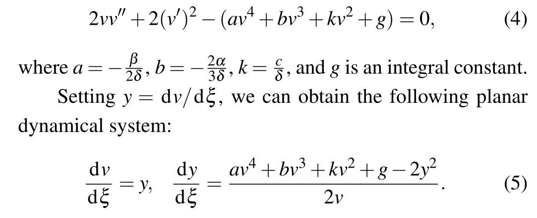
From Refs. [19–24], we know that a solitary wave solution to Eq. (4) corresponds to a homoclinic orbit of system(5), a peakon (or a periodic cusp wave) solution to Eq. (4)corresponds to a heteroclinic orbit (or the so-called connecting orbit)of system(5). Similarly, a periodic orbit of system(5)corresponds to a smooth periodic wave solution to Eq.(4).Thus, to investigate all possible solitary waves, peakons and periodic waves of Eq.(4),we need to find all homoclinic,heteroclinic and periodic annuli of system(5), which depend on the system parametersa,b,kandg. For simplicity, we only investigate the case ofa <0 in this paper. The case ofa >0 can be considered similarly,we omit it here.
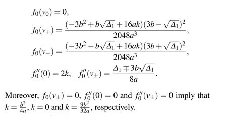
where?1=9b2?32ak. Additionally,
2. Bifurcation sets and phase portraits of system(5)
Using the transformation dξ=2vdτ,we obtain the associated Hamiltonian system of system(5)
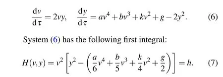
For a fixedh,the level curveH(v,y)=hdefined by Eq.(7)determines a set of invariant curves of system(6),which contains different branches of curves. Ashvaries, it defines different families of orbits of system(6)with different dynamical behaviors.
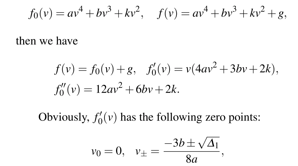
Let
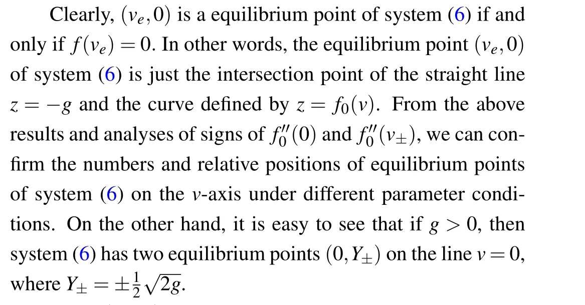
LetM(ve,ye) be the coefficient matrix of the linearized system of Eq.(6)at equilibrium point(ve,ye)andJ(ve,ye)=det(M(ve,ye)),we have
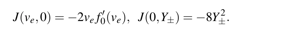
For an equilibrium point(ve,ye)of system(6),we know that(ve,ye)is a saddle point ifJ(ve,ye)<0, a center point ifJ(ve,ye)>0,a cusp ifJ(ve,ye)=0 and the Poincar′e index of(ve,ye)is zero.
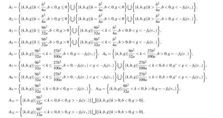
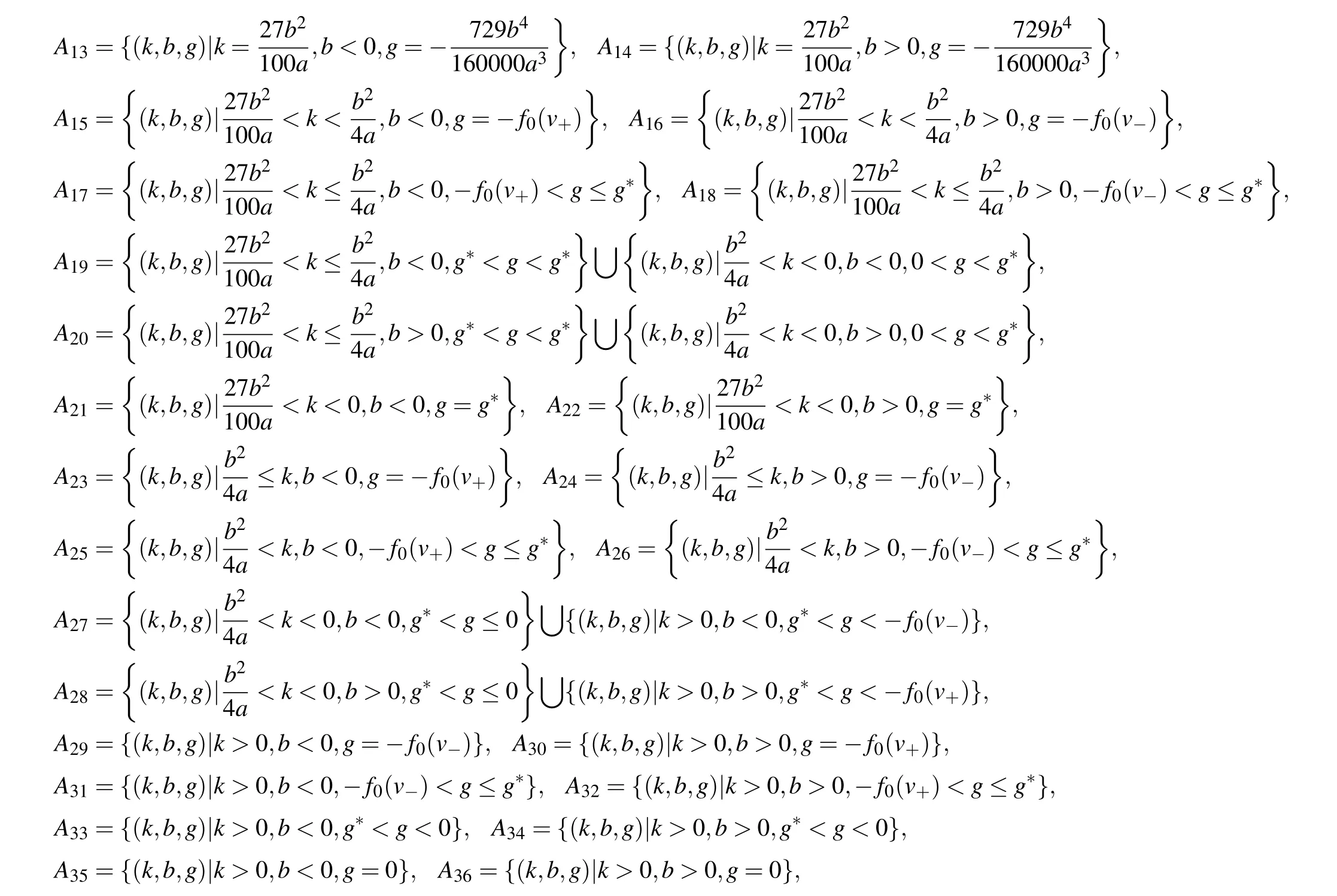
For fixedaandb,using the properties of the equilibrium points and the approach of dynamical system,[19–24]we can obtain the following bifurcation curves of system(6):
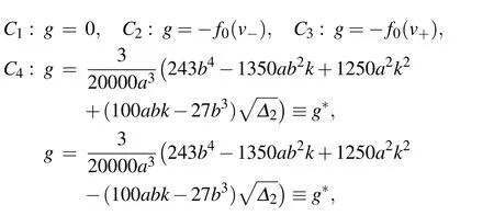
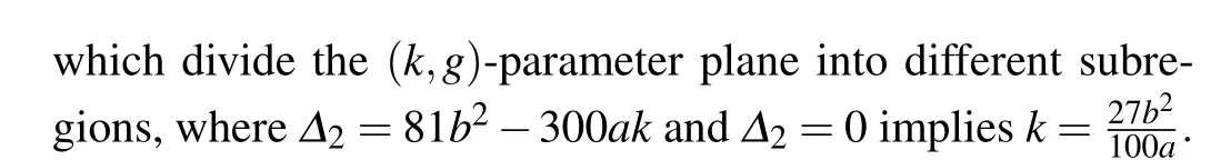
Since both systems (5) and (6) have the same first integral (7), the two systems have the same topological phase portraits except the straight linev=0. Therefore we can obtain the bifurcation sets and phase portraits of system(5)from those of system(6).
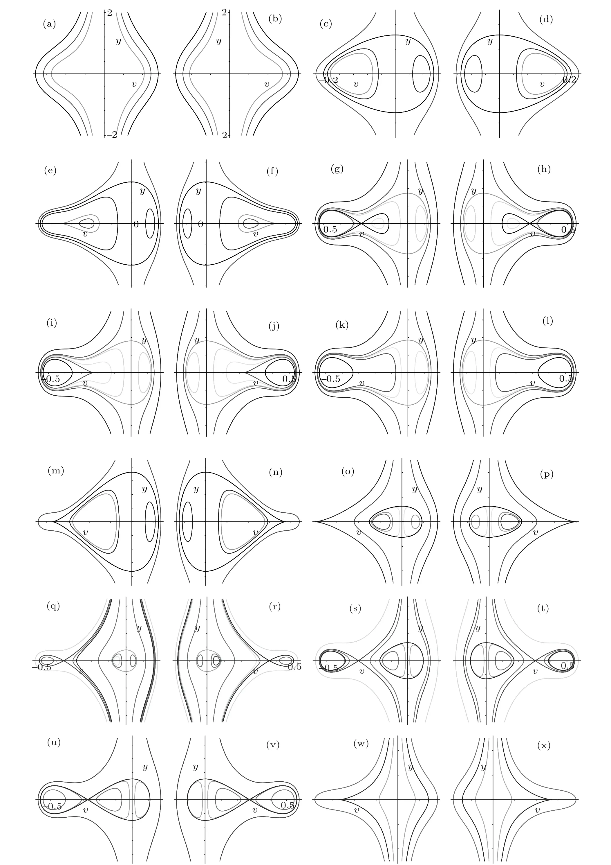
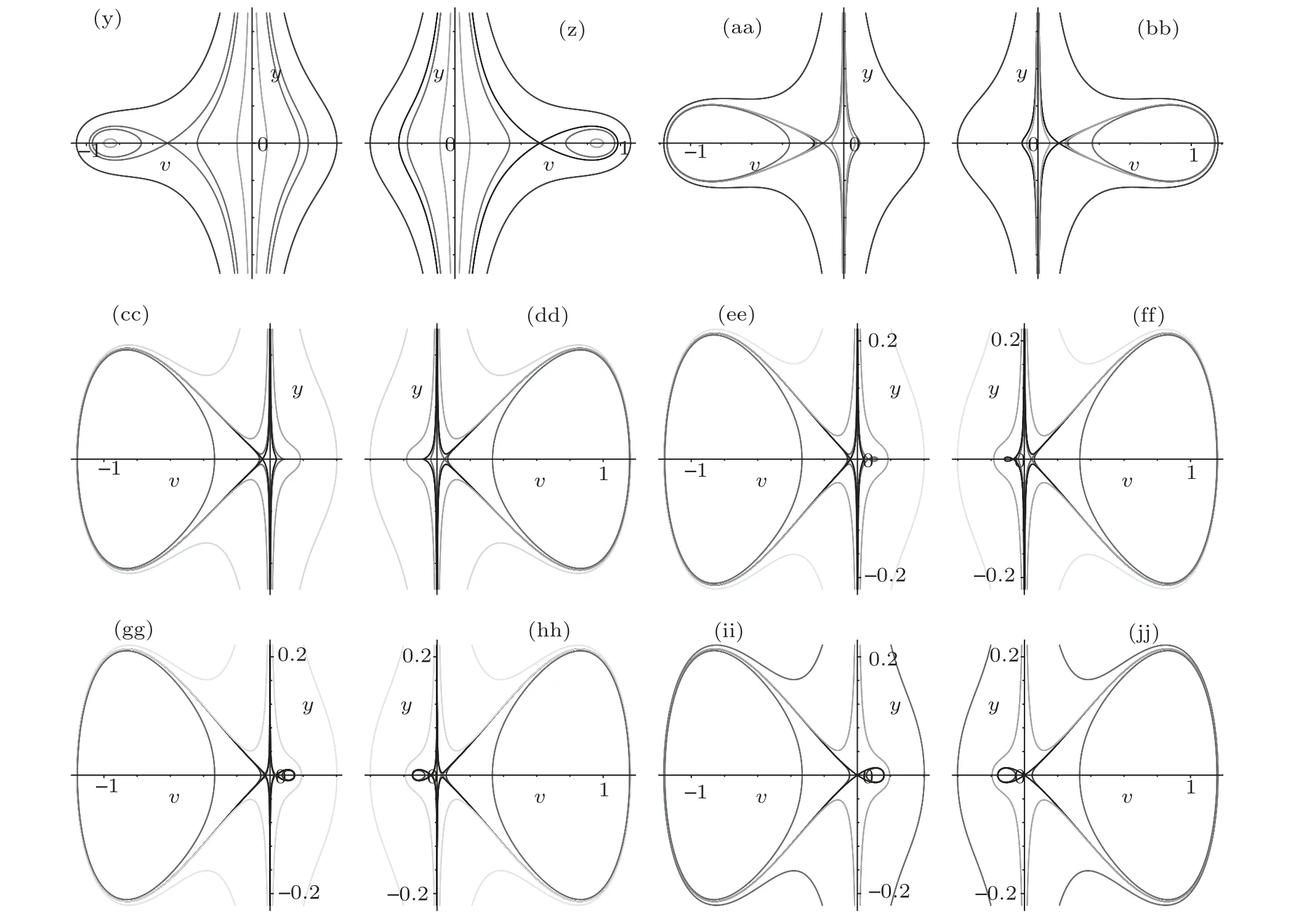
Fig.1. Bifurcation sets and phase portraits of system(5)when a <0.Parameters:(a)(k,b,g)∈A1.(b)(k,b,g)∈A2.(c)(k,b,g)∈A3.(d)(k,b,g)∈A4.(e)(k,b,g)∈A5. (f)(k,b,g)∈A6. (g)(k,b,g)∈A7. (h)(k,b,g)∈A8. (i)(k,b,g)∈A9. (j)(k,b,g)∈A10. (k)(k,b,g)∈A11. (l)(k,b,g)∈A12. (m)(k,b,g)∈A13. (n)(k,b,g)∈A14. (o)(k,b,g)∈A15. (p)(k,b,g)∈A16. (q)(k,b,g)∈A17. (r)(k,b,g)∈A18. (s)(k,b,g)∈A19. (t)(k,b,g)∈A20. (u)(k,b,g)∈A21.(v)(k,b,g)∈A22.(w)(k,b,g)∈A23.(x)(k,b,g)∈A24.(y)(k,b,g)∈A25.(z)(k,b,g)∈A26.(aa)(k,b,g)∈A27.(bb)(k,b,g)∈A28.(cc)(k,b,g)∈A29. (dd)(k,b,g)∈A30. (ee)(k,b,g)∈A31. (ff)(k,b,g)∈A32. (gg)(k,b,g)∈A33. (hh)(k,b,g)∈A34. (ii)(k,b,g)∈A35. (jj)(k,b,g)∈A36.
Let
we show that bifurcation sets and phase portraits of system(5)in Fig.1.
3. Exact explicit solitary wave and periodic wave solutions to Eq.(1)
According to Fig. 1 and the approach of dynamical system,[19–24]we present some exact explicit solitary wave and periodic wave solutions to Eq.(1)as follows.
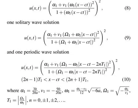
Proposition 3.1. Whena <0,(k,b,g)∈A13,Eq.(1)has oneω-shape solitary wave solution
Substituting Eqs.(11)–(13)into dv/dξ=yand integrating them along the homoclinic orbit, the heteroclinic orbits,respectively,we have
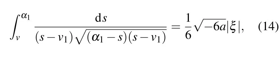
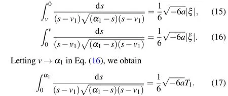
Completing the integrals in Eqs. (14)–(17), we can obtain one solitary wave solution, one peakon solution and one periodic cusp wave solution to Eq.(4)as follows:
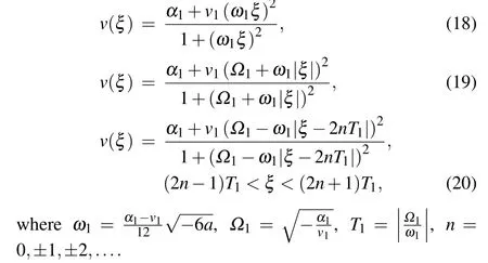
From Eqs.(2),(18)–(20),we can obtain oneω-shape solitary wave solution,one solitary wave solution and one periodic wave solution to Eq.(1)as Eqs.(8)–(10),respectively.
The proof of Proposition 3.1 is completed.
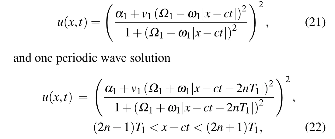
Proposition 3.2. Whena <0,(k,b,g)∈A14,Eq.(1)has oneω-shape solitary wave solution as Eq. (8), one solitary wave solution
Substituting Eqs.(23)–(25)into dv/dξ=yand integrating them along the homoclinic orbit, the heteroclinic orbits,respectively,we have
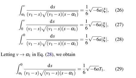
Completing the integrals in Eqs.(26)–(29),we can obtain one solitary wave solution to Eq.(4)as Eq.(18), one peakon solution and one periodic cusp wave solution to Eq.(4)as follows:
From Eqs.(2),(18),(30)and(31),we can obtain oneωshape solitary wave solution, one solitary wave solution and one periodic wave solution to Eq. (1) as Eqs. (8), (21) and(22),respectively.
The proof of Proposition 3.2 is completed.
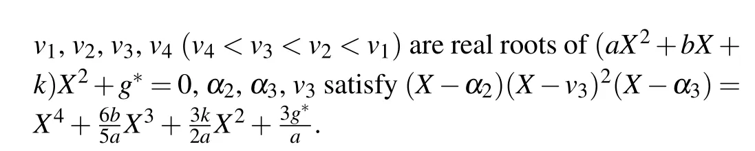
Proposition 3.3. Whena <0,(k,b,g)∈A21,Eq.(1)has oneω-shape solitary wave solution
two solitary wave solutions
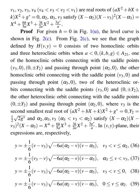
Substituting Eqs.(36)–(39)into dv/dξ=yand integrating them along the homoclinic orbits, the heteroclinic orbits,respectively,we have
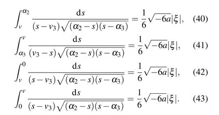
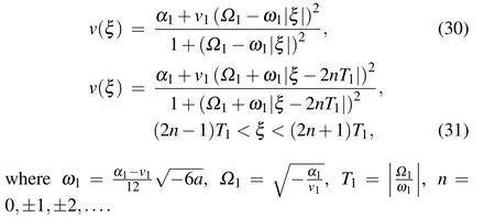
Lettingv →α2in Eq.(43),we obtain
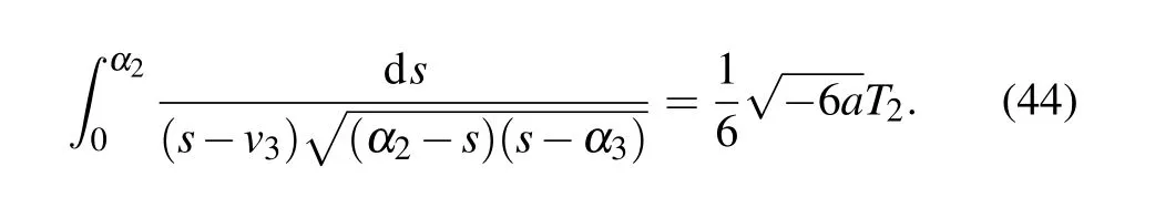
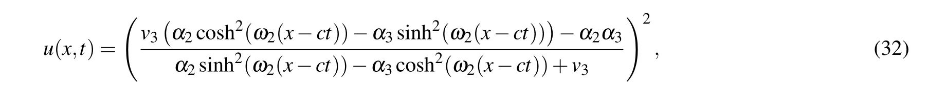
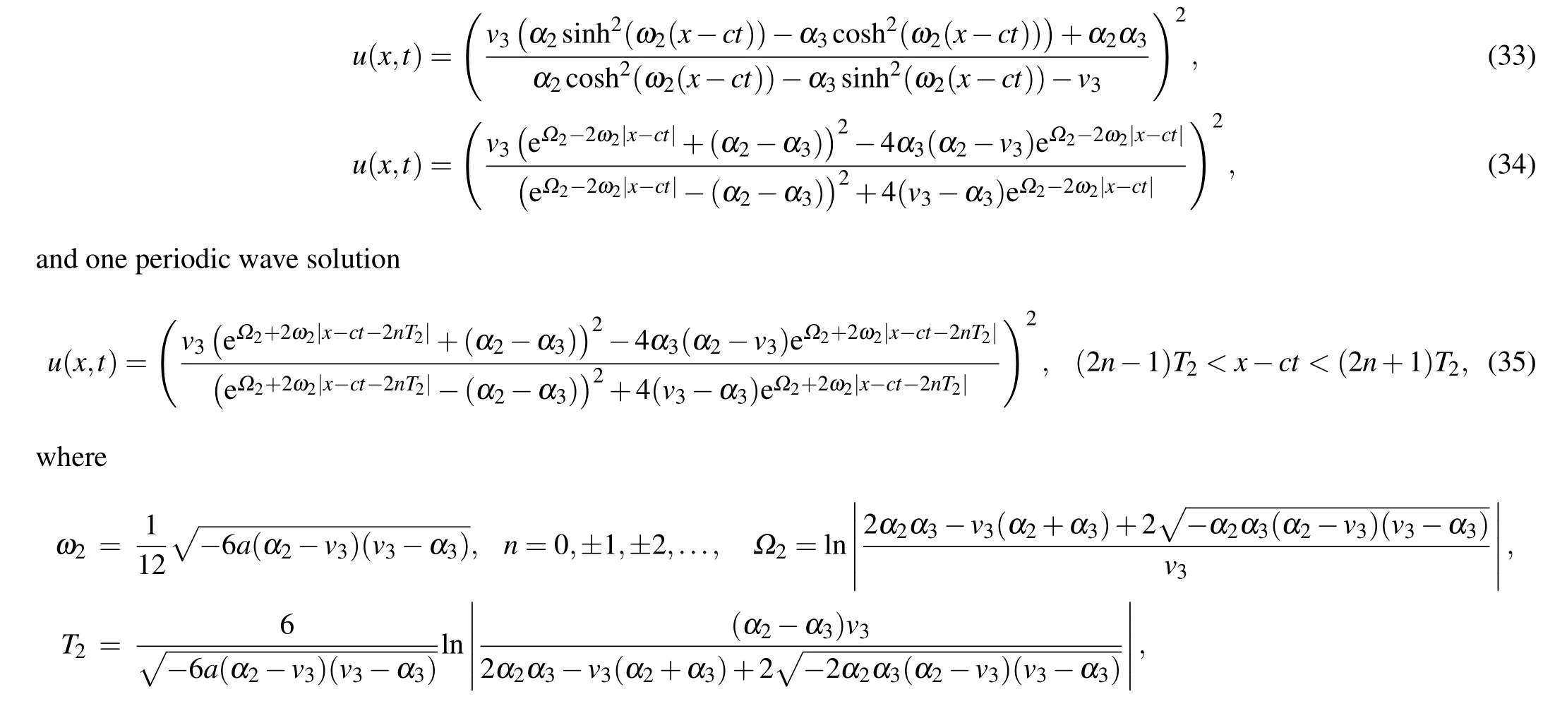
Completing the integrals in Eqs. (40)–(44), we can obtain two solitary wave solutions,one peakon solution and one periodic cusp wave solution to Eq.(4)as follows:

where
From Eqs. (2), (45)–(48), we obtain oneω-shape solitary wave solution, two solitary wave solutions and one periodic wave solution to Eq.(1)as Eqs.(32)–(35),respectively.
The proof of Proposition 3.3 is completed.
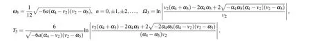
Proposition 3.4. Whena <0,(k,b,g)∈A22,Eq.(1)has oneω-shape solitary wave solution
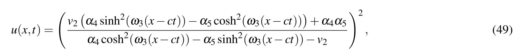
two solitary wave solutions
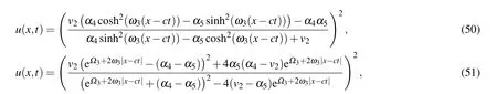
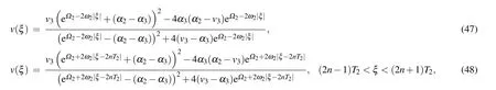
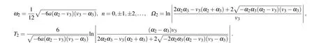
and one periodic wave solution
where
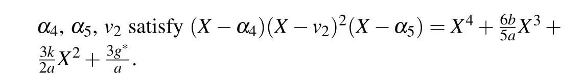

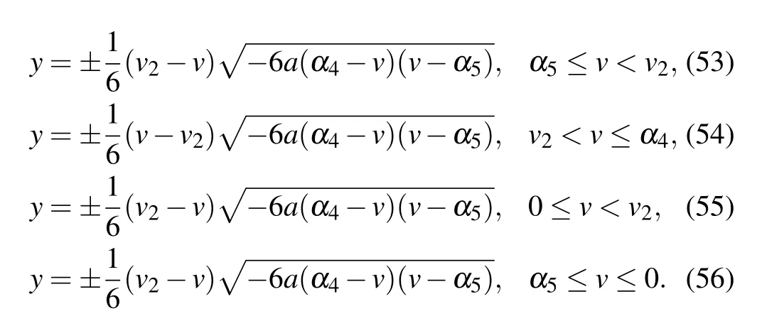
Substituting Eqs.(53)–(56)into dv/dξ=yand integrating them along the homoclinic orbits, the heteroclinic orbits,respectively,we have
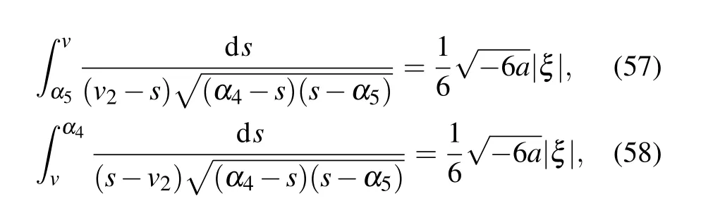
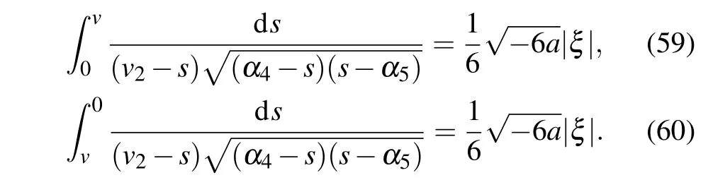
Lettingv →α5in Eq.(60),we obtain
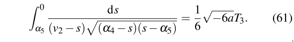
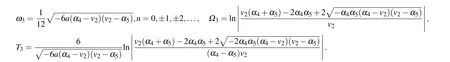
Completing the integrals in Eqs. (57)–(61), we can obtain two solitary wave solutions,one peakon solution and one periodic cusp wave solution to Eq.(4)as follows:
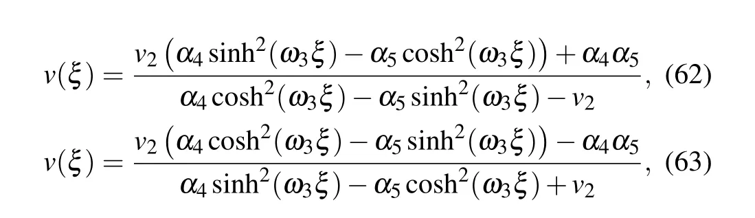
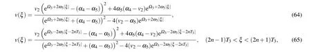
where
From Eqs.(2),(62)–(65),we obtain oneω-shape solitary wave solution, two solitary wave solutions and one periodic wave solution to Eq.(1)as Eqs.(49)–(52),respectively.
The proof of Proposition 3.4 is completed.
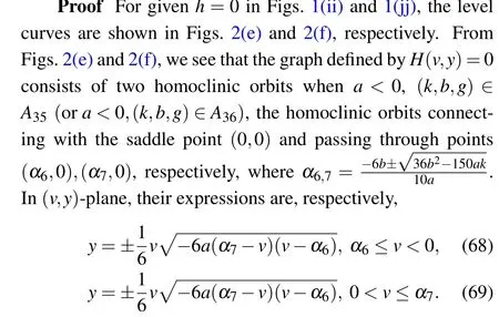
Substituting Eqs. (68) and (69) into dv/dξ=yand integrating them along the homoclinic orbits, respectively, we have
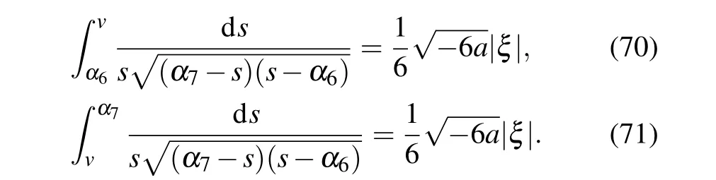
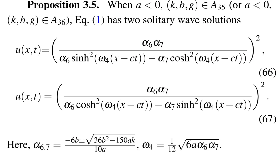
Completing the integrals in Eqs. (70) and (71), we can obtain two solitary wave solutions to Eq.(4)as follows:
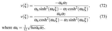
From Eqs.(2),(72)and(73),we obtain two solitary wave solutions to Eq.(1)as Eqs.(66)and(67).
The proof of Proposition 3.5 is completed.
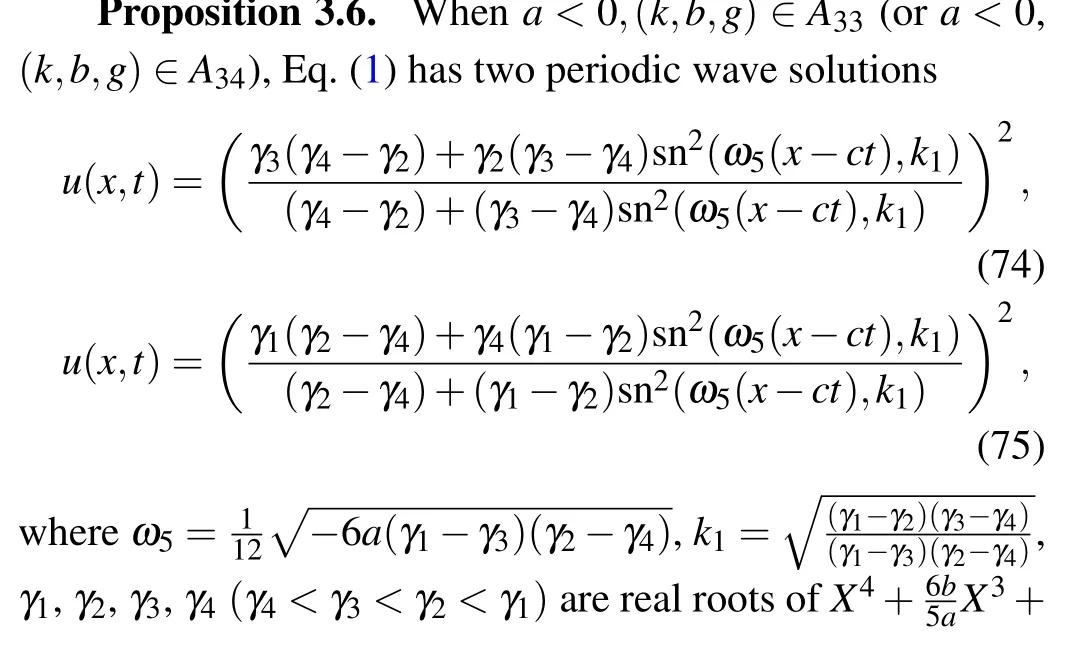
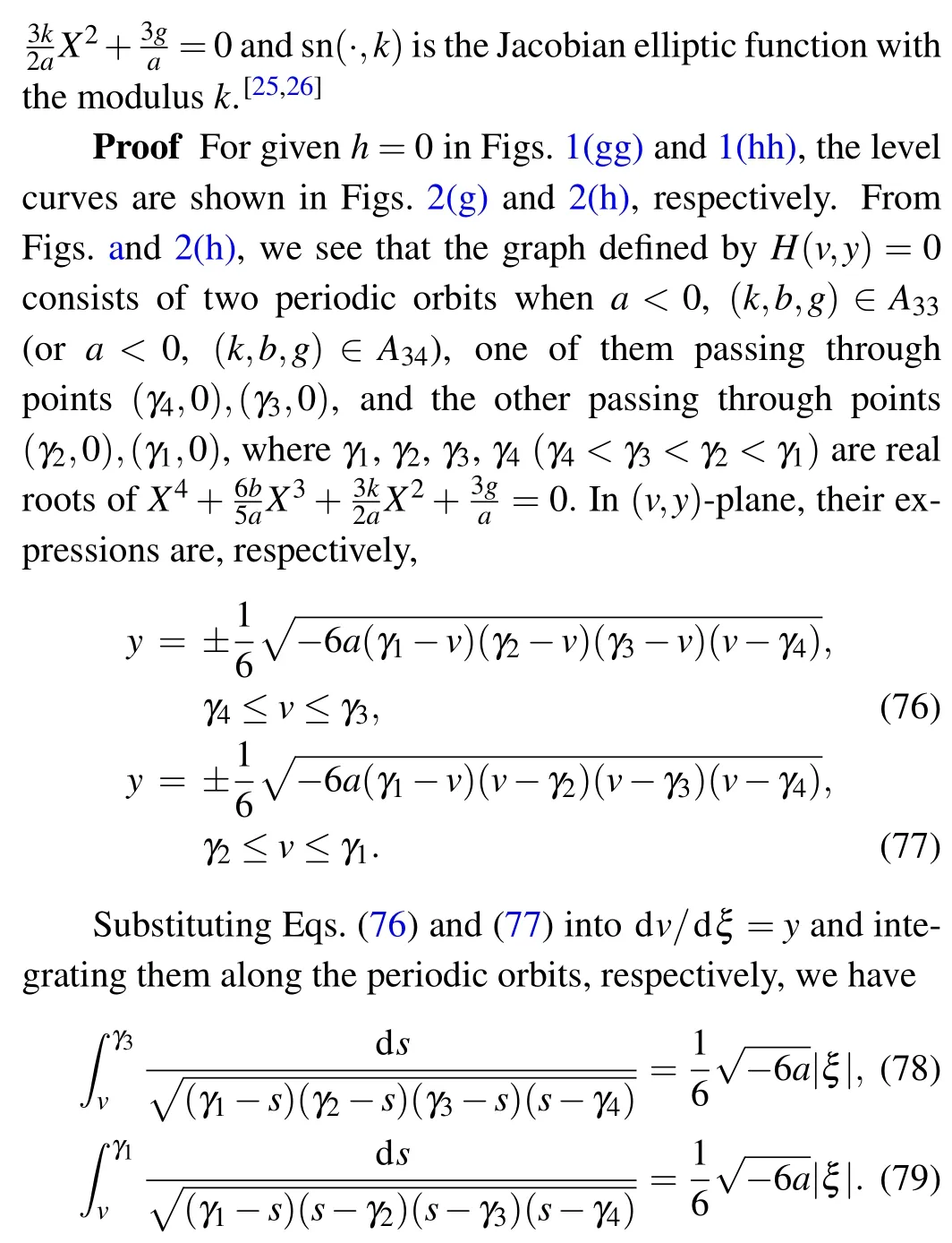
Completing the integrals in Eqs. (78) and (79), we can obtain two periodic wave solutions to Eq.(4)as follows:
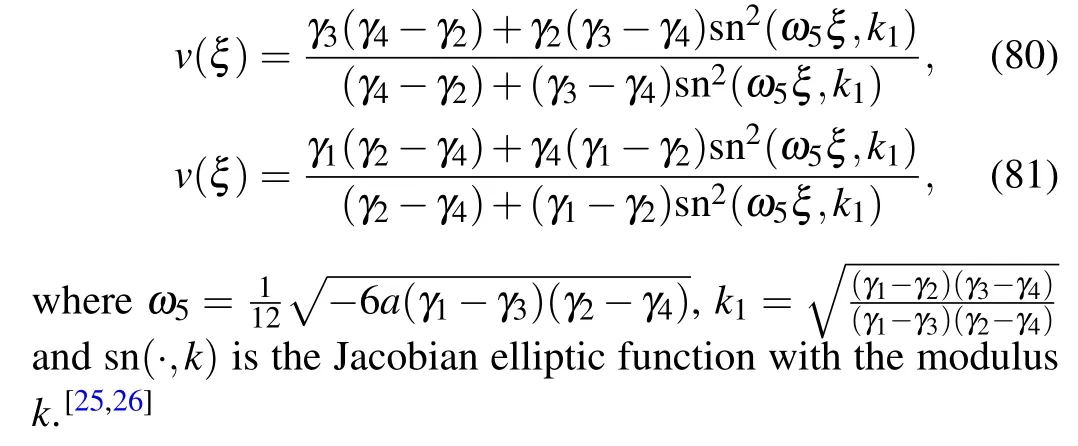
From Eqs.(2),(80)and(81),we obtain two periodic wave solutions to Eq.(1)as Eqs.(74)and(75).
The proof of Proposition 3.6 is completed.
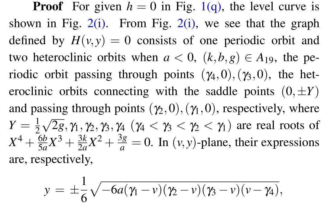
Proposition 3.7. Whena <0,(k,b,g)∈A19,Eq.(1)has a periodic wave solution as Eq.(74). Whena <0, (k,b,g)∈A20,Eq.(1)has a periodic wave solution as Eq.(75).
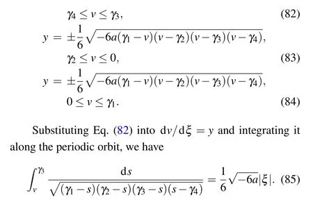
Completing the integral in Eq. (85), we can obtain one periodic wave solution to Eq. (4) as Eq. (80). From Eqs. (2)and (80), we obtain one periodic wave solution to Eq. (1) as Eq.(74).
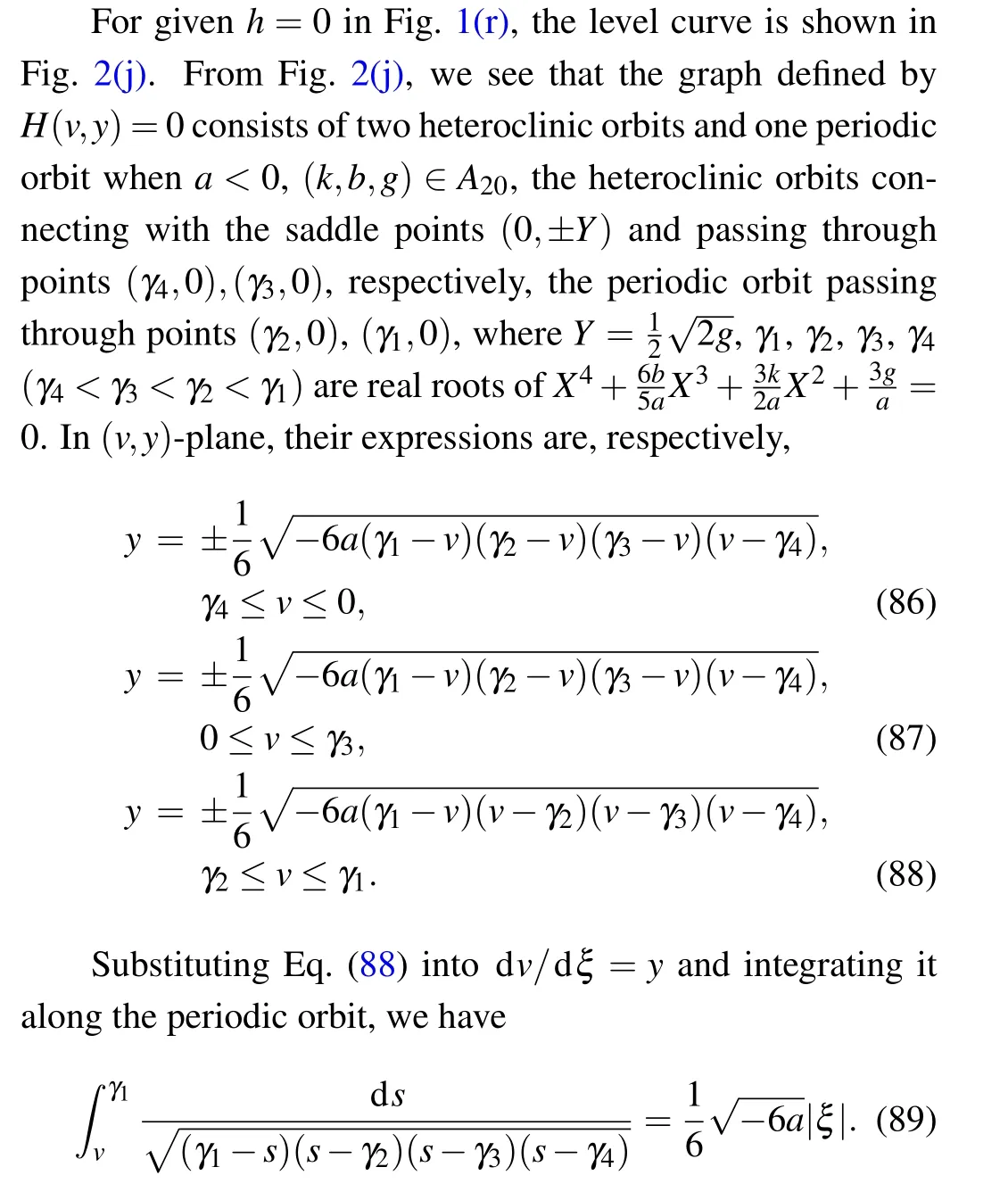
Completing the integral in Eq. (89), we can obtain one periodic wave solution to Eq. (4) as Eq. (81). From Eqs. (2)and (81), we obtain one periodic wave solution to Eq. (1) as Eq.(75).
The proof of Proposition 3.7 is completed.
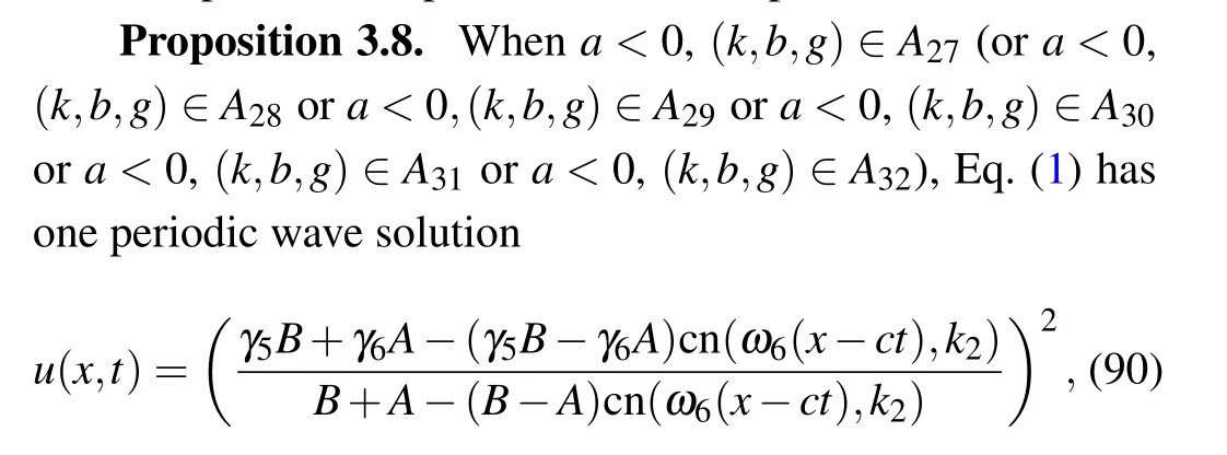
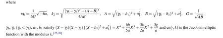
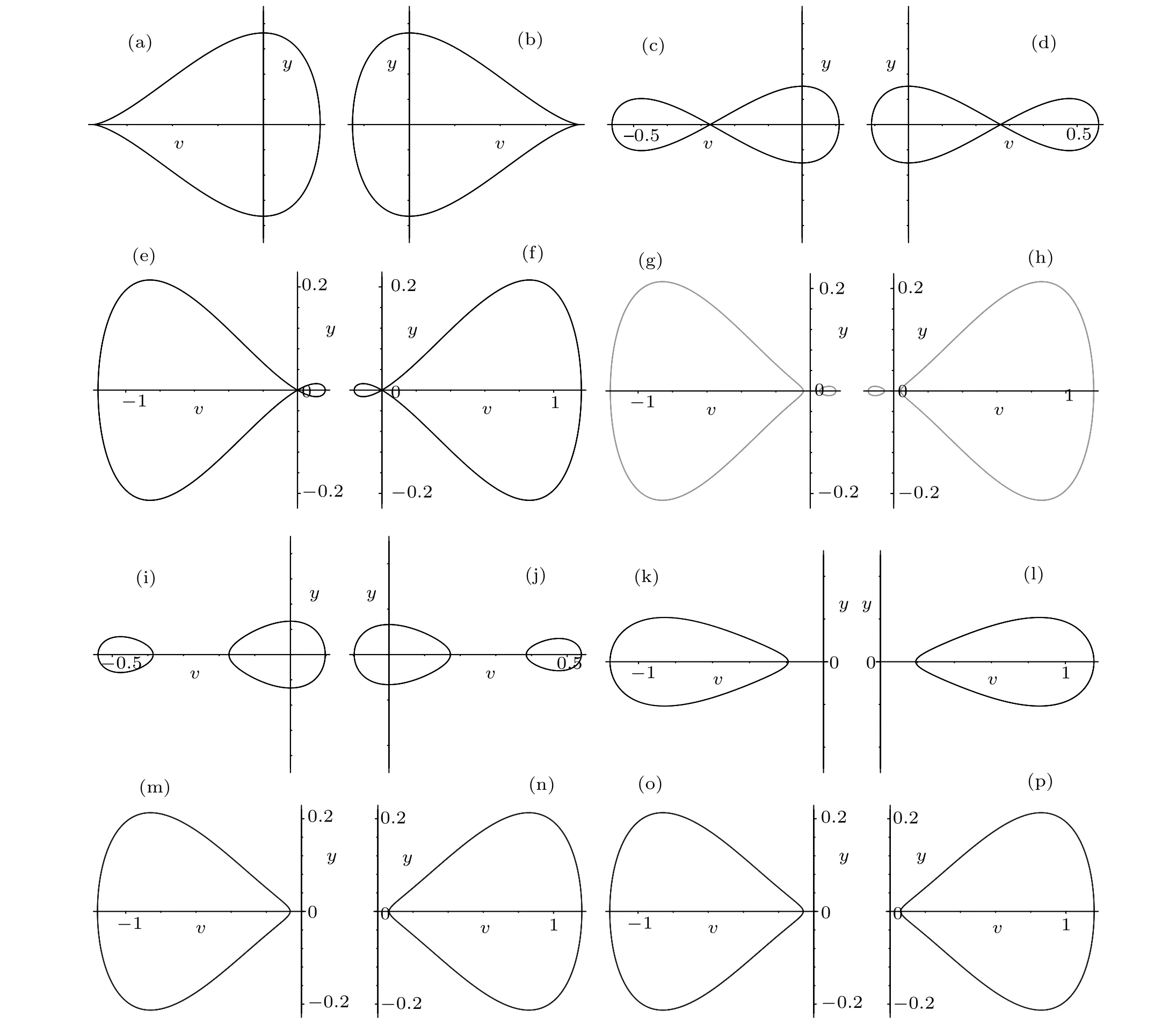
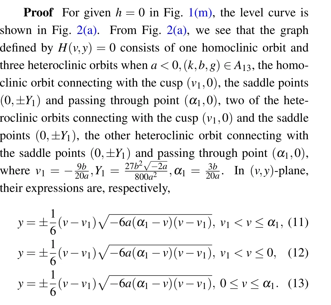
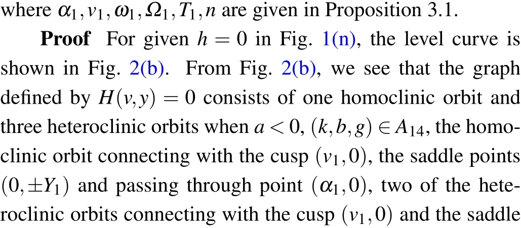
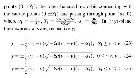
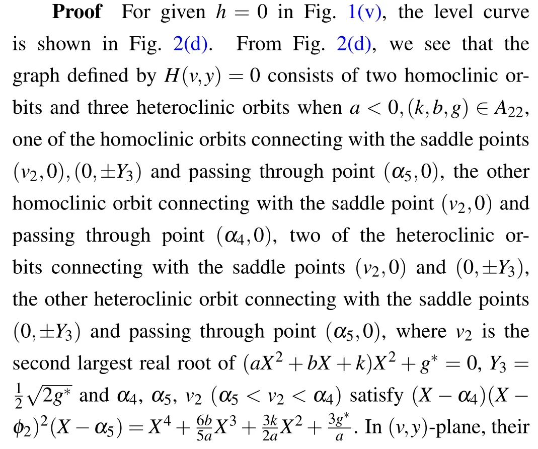
Fig. 2. The level curves defined by H(v,y)=0 when a <0. Parameters: (a) (k,b,g)∈A13. (b) (k,b,g)∈A14. (c) (k,b,g)∈A21. (d)(k,b,g)∈A22.(e)(k,b,g)∈A35.(f)(k,b,g)∈A36.(g)(k,b,g)∈A33.(h)(k,b,g)∈A34.(i)(k,b,g)∈A19.(j)(k,b,g)∈A20.(k)(k,b,g)∈A27.(l)(k,b,g)∈A28. (m)(k,b,g)∈A29. (n)(k,b,g)∈A30. (o)(k,b,g)∈A31. (p)(k,b,g)∈A32.
Proof For givenh= 0 in Figs. 1(aa)–1(ff), the level curves are shown in Figs. 2(k)–2(p), respectively. From Figs. 2(k)–2(p), we see that the graph defined byH(v,y)=0 consists of one periodic orbit whena <0, (k,b,g)∈A27(ora <0,(k,b,g)∈A28ora <0,(k,b,g)∈A29ora <0,(k,b,g)∈A30ora <0,(k,b,g)∈A31ora <0,(k,b,g)∈A32),the periodic orbit passing through points(γ6,0),(γ5,0).In(v,y)-plane,its expression is
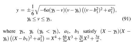
Substituting Eq. (91) into dv/dξ=yand integrating it along the periodic orbit,we have
Completing the integral in Eq. (92), we can obtain one periodic wave solution to Eq.(4)as follows:
From Eqs.(2)and(93),we obtain one periodic wave solution to Eq.(1)as Eq.(90).
The proof of Proposition 3.8 is completed.
4. Numerical simulations
In this section, we simulate the analytical results along with above details of the analysis.
Under the parameter conditionsa <0,(k,b,g)∈A13,we can draw the profiles of Eqs.(18)–(20)and Eqs.(8)–(10). For example,takinga=?1.2,b=?1.5,the profiles of Eqs.(18)–(20) and Eqs. (8)–(10) are shown in Figs. 3(a)–3(f), respectively.
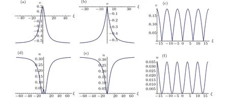
Fig.3. Profiles of Eqs.(18)–(20)and Eqs.(8)–(10).
Under the parameter conditionsa <0,(k,b,g)∈A14,we can draw the profiles of Eqs.(18),(30), (31),(8),(21)and(22).For example, takinga=?1.2,b=1.5, the profiles of Eqs. (18), (30), (31), (8), (21) and (22) are shown in Figs. 4(a)–4(f),respectively.
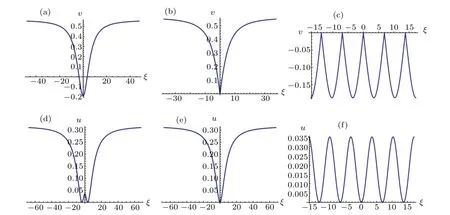
Fig.4. Profiles of Eqs.(18),(30),(31),(8),(21)and(22).

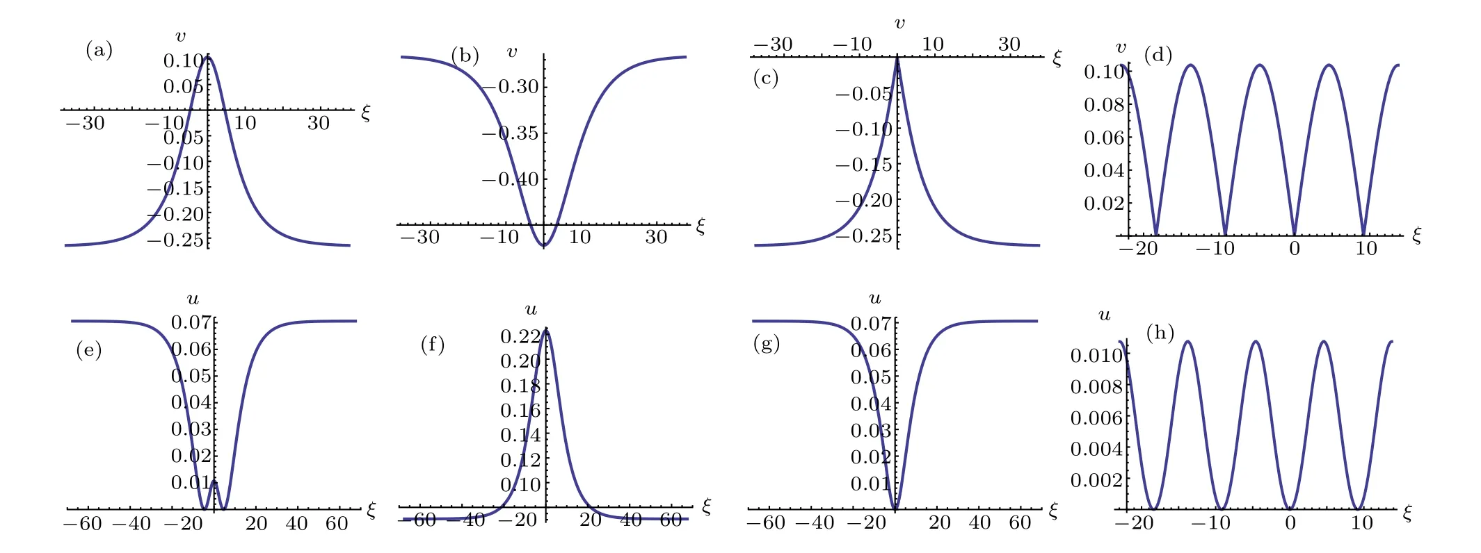
Fig.5. Profiles of Eqs.(45)–(48)and Eqs.(32)–(35).
Under the parameter conditionsa <0,(k,b,g)∈A35(ora <0, (k,b,g)∈A36) we can draw the profiles of Eqs. (72),(73),(66)and(67). For example,takinga=?1.5,b=?1.2,k=0.5,the profiles of Eqs.(72),(73),(66),and(67)are shown in Figs.7(a)–7(d),respectively.
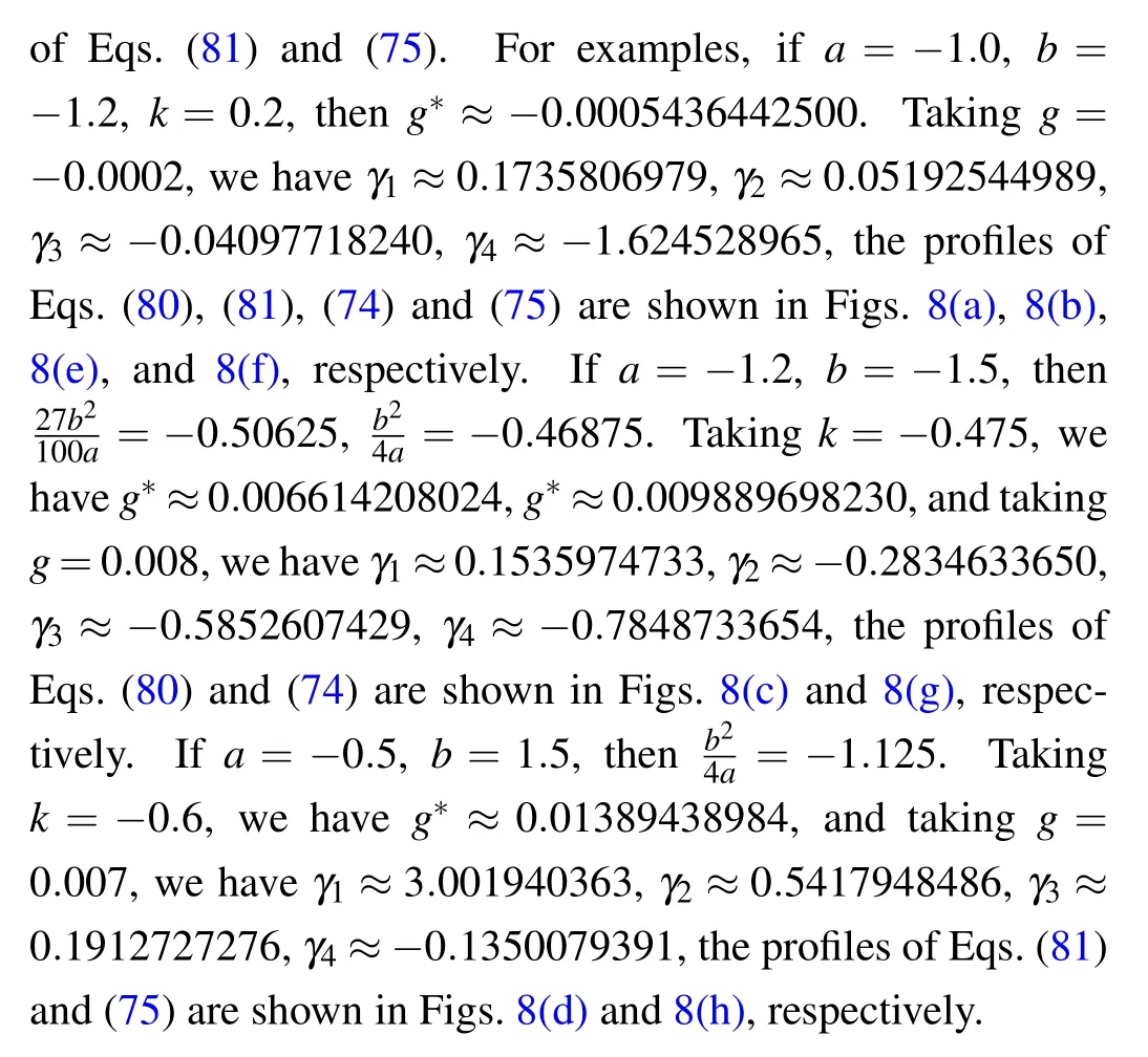
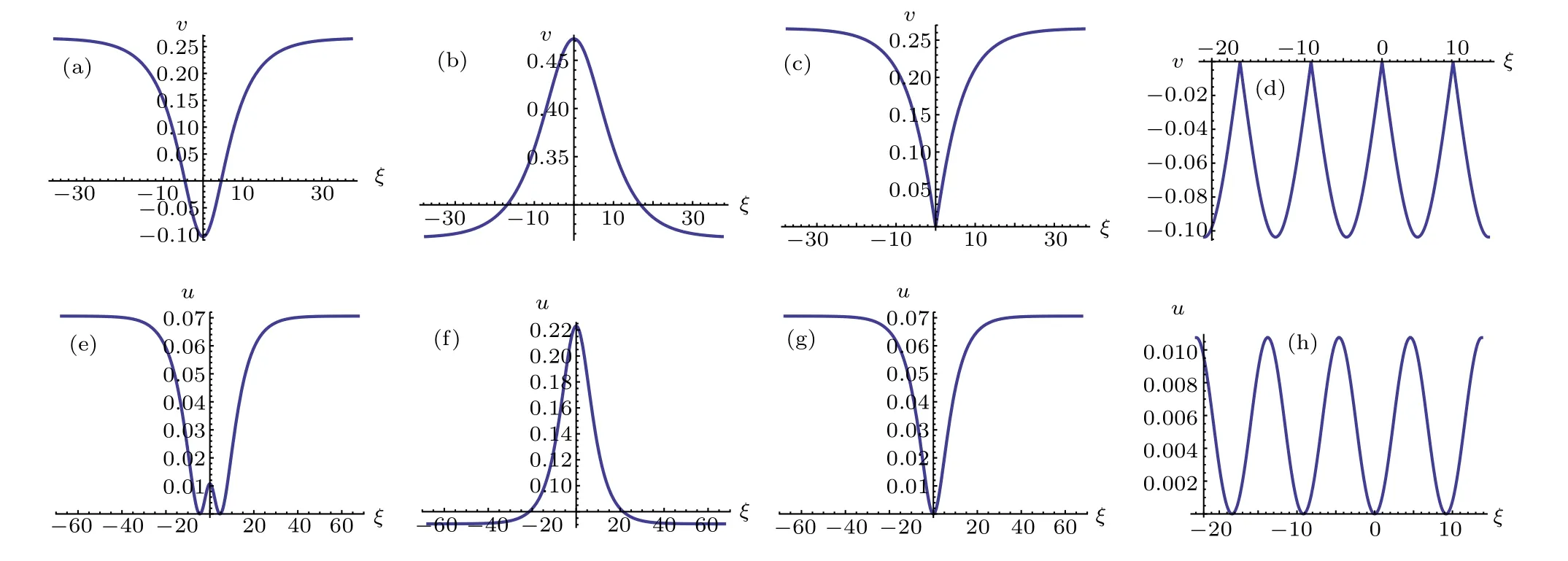
Fig.6. Profiles of Eqs.(62)–(65)and Eqs.(49)–(52).
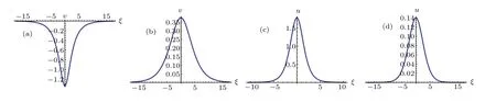
Fig.7. Profiles of Eqs.(72),(73),(66),and(67).
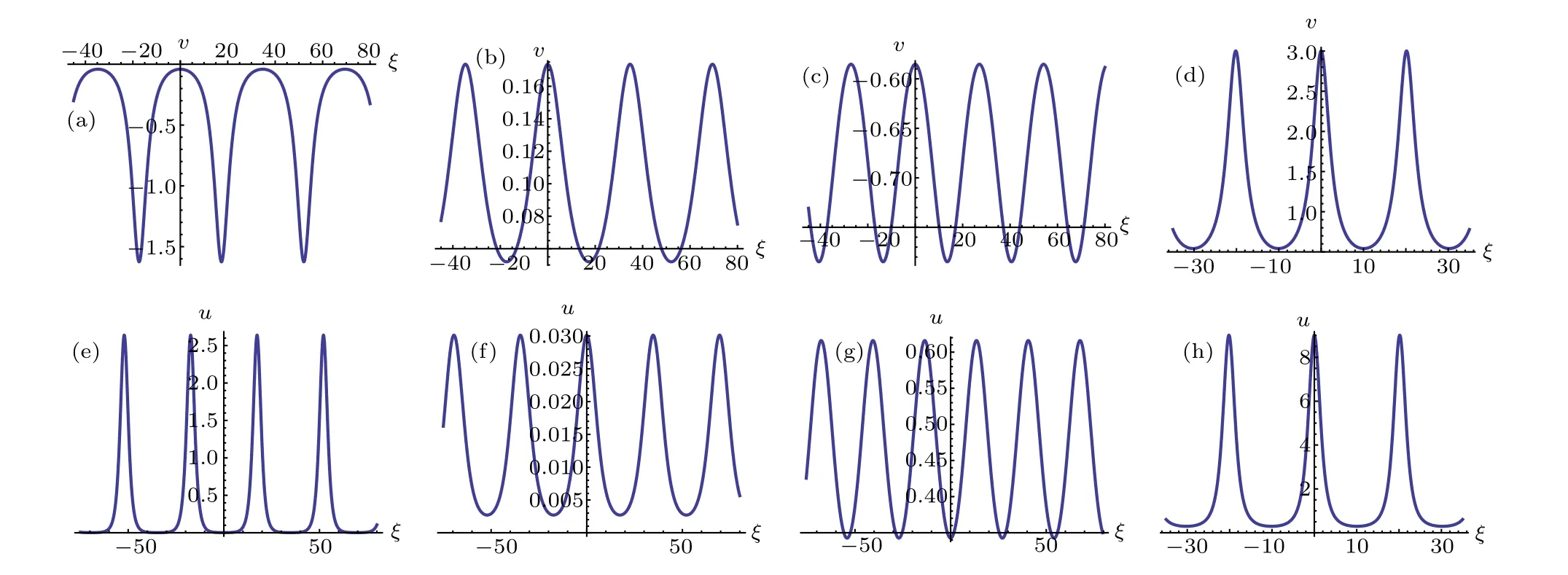
Fig.8. Profiles of Eqs.(80),(81),(74)and(75).
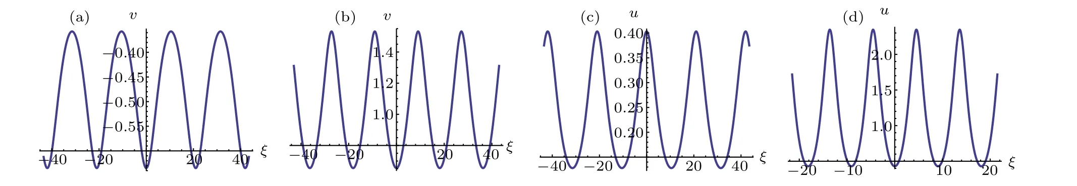
Fig.9. Profiles of Eqs.(93)and(90).
5. Conclusion
In summary,we have investigated the existences and dynamical behaviors of exact explicit solitary wave and periodic wave solutions of the Schamel–Korteweg–de Vries equation (1) in different regions of the parametric space. Some exact explicit solitary wave and periodic wave solutions to Eq.(1)whena <0,(k,b,g)∈A13(ora <0,(k,b,g)∈A14ora <0,(k,b,g)∈A21ora <0,(k,b,g)∈A22ora <0,(k,b,g)∈A35ora <0,(k,b,g)∈A36ora <0,(k,b,g)∈A33ora <0,(k,b,g)∈A34ora <0,(k,b,g)∈A19ora <0,(k,b,g)∈A20ora <0,(k,b,g)∈A27ora <0,(k,b,g)∈A28ora <0,(k,b,g)∈A29ora <0,(k,b,g)∈A30ora <0,(k,b,g)∈A31ora <0,(k,b,g)∈A32) are given in Propositions 3.1–3.8.Comparing with the results of[11–18], we obtain some new traveling wave solutions such asω-shape solitary wave solutions (8), (32), (49), solitary wave solutions (9), (21), (34),(51), and periodic wave solutions (10), (22), (35), (52), etc.Obviously, there are still many works of Eq. (1) for studying in future,for examples,does the Eq.(1)exist loop soliton and periodic loop soliton solutions? How to obtain more nontraveling wave solutions to Eq. (1)? We will study Eq. (1)further.

- Chinese Physics B的其它文章
- Coarse-grained simulations on interactions between spectrins and phase-separated lipid bilayers?
- Constraints on the kinetic energy of type-Ic supernova explosion from young PSR J1906+0746 in a double neutron star candidate?
- Computational model investigating the effect of magnetic field on neural–astrocyte microcircuit?
- Gas sensor using gold doped copper oxide nanostructured thin films as modified cladding fiber
- Suppression of ferroresonance using passive memristor emulator
- Suppression of ice nucleation in supercooled water under temperature gradients