CONTINUOUS TIME MIXED STATE BRANCHING PROCESSES AND STOCHASTIC EQUATIONS?

Shukai CHEN(陳舒凱) Zenghu LI(李增滬)

Laboratory of Mathematics and Complex Systems,School of Mathematical Sciences,Beijing Normal University,Beijing 100875,China

E-mail:skchen@mail.bnu.edu.cn;lizh@bnu.edu.cn

Abstract A continuous time and mixed state branching process is constructed by a scaling limit theorem of two-type Galton-Watson processes.The process can also be obtained by the pathwise unique solution to a stochastic equation system.From the stochastic equation system we derive the distribution of local jumps and give the exponential ergodicity in Wasserstein-type distances of the transition semigroup.Meanwhile,we study immigration structures associated with the process and prove the existence of the stationary distribution of the process with immigration.

Key words mixed state branching process;weak convergence;stochastic equation system;Wasserstein-type distance;stationary distribution.

1 Introduction

Branching processes were introduced as probabilistic models describing the evolution of populations.The study of branching processes was initiated by Bienaym′e(1845)and Galton and Watson(1874),independently,and the processes were referred to as discrete time and discrete state branching processes(GW-processes).To increase speci ficity,several naturally generalized processes including continuous time discrete state branching processes(DB-processes)with or without immigration and continuous time continuous state branching processes(CB-processes)with or without immigration,were subsequently introduced and studied by researchers.

The DB-processes are continuous time discrete state Markov processes with lifetimes that are independent and with exponentially distributed random variables.There have been many works on DB-processes,including ones pertaining to their construction,to the properties of moments,to limit theorems and so on;we refer to[1]for the details regarding these.The application of stochastic equations to branching processes has been developed in recent decades.Let N={0,1,2,···}and let?(·)=be a counting measure on N.Let X={Xt:t≥0}be a DB-process with immigration with a branching rate c>0,offspring distribution(pi:i∈N),an immigration rate η>0 and immigration distribution(qi:i∈N).The two distributions satisfy<∞.It is known that X can be obtained as a pathwise unique strong solution to the stochastic equation

where X0is a random variable taking values in N,M(ds,dz,du)is a Poisson random measure on(0,∞)×N×(0,∞)with intensity measure cpzds?(dz)du,N(ds,dz)is a Poisson random measure on(0,∞)×N with intensity measure ηqzds?(dz),and X0,M(ds,dz,du)and N(ds,dz)are independent of each other.In particular,if η≡0,qz≡0 for all z∈N,this reduces things to the DB-process.Moreover,here and in the sequel,we understand that for any b≥a≥0,

CB-processes were first introduced in[16],to model the random evolution of large population dynamics.Denoting the law on D([0,∞),[0,∞))by Pxfor each initial value x≥0,the branching property of processes can be described by Px+y=Px?Py.The semigroup of CB-processes with immigration(CBI-processes)(Qt)t≥0can be characterized uniquely by the Laplace transform

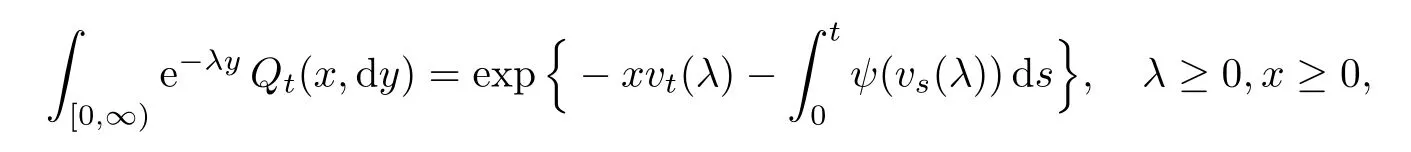
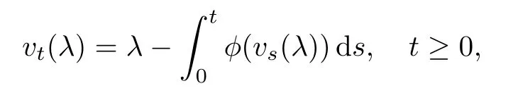
and the branching mechanism φ and immigration mechanism ψ de fined on[0,∞)take the form of

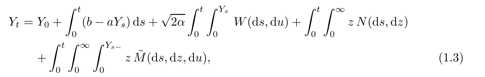
where Y0is a random variable taking values in R+,W(ds,du)is a time-space white noise with intensity measure dsdu,M(ds,dz,du)is a Poisson random measure on(0,∞)3with intensity measure dsm(dz)du,N(ds,dz)is a Poisson random measure on(0,∞)2with intensity measure dsn(dz)and(ds,dz,du)=M(ds,dz,du)?dsm(dz)du is the compensated measure of M(ds,dz,du).Moreover,Y0,W,M and N are independent of each other.We mention that the moment conditionz n(dz)<∞was removed in[13].The sample paths of Y can also be obtained as a unique strong solution to a stochastic equation driven by Brownian motions and Poisson random measures.One finds that the formulation(1.3)is nicer for analysing the flows of CBI-processes and other applications;see[6]for the speci fic construction.We refer to[3,5,6,13,23,25,30]for more on this approach and further properties of the above stochastic equations.Based on the stochastic equations established above,[14]studied the explicit expression of the distribution of jumps.[17]gave the criteria for the existence of general moments for CB-processes with or without immigration under a more general branching mechanism,where the characterization of the processes in terms of stochastic equations plays an essential role,and[18]extended those results to the processes in Lvy random environments.Some applications for finance can be found in[19].A two-type CBI-process obtained as a unique strong solution of a stochastic equation system was studied in[28,29].

We can rewrite(1.3)without an immigration part by extending the M to a Poisson random measure denoted again by M on(0,∞)3×N with intensity dsm(dz)du?(dk)for some λ>0 as follows:

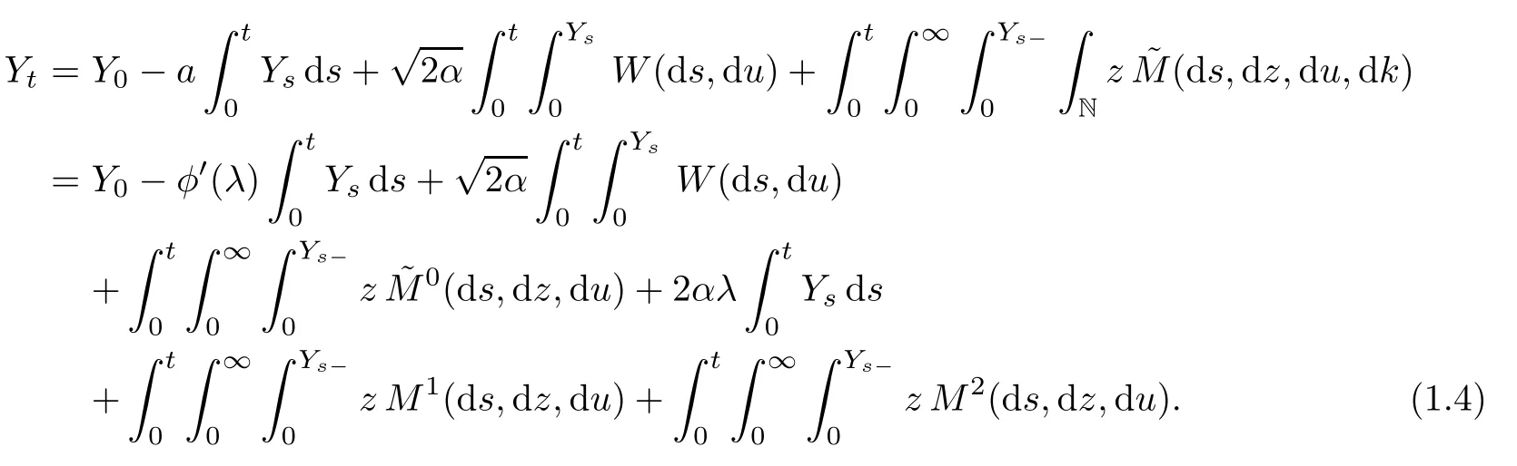
Here,M0(ds,dz,du)=M(ds,dz,du,{k=0})and

Recently,[9]gave another SDE-type description for one-dimensional CB-processes based on(1.4)with a<0,λ≥λ?;here λ?is the unique root of φ on(0,∞).One of the results in[9]shows that the last three integrals on the right-hand side of(1.4)are identi fied with the mass that immigrates from the skeleton construction.More precisely,the following stochastic equation system has a unique strong solution:

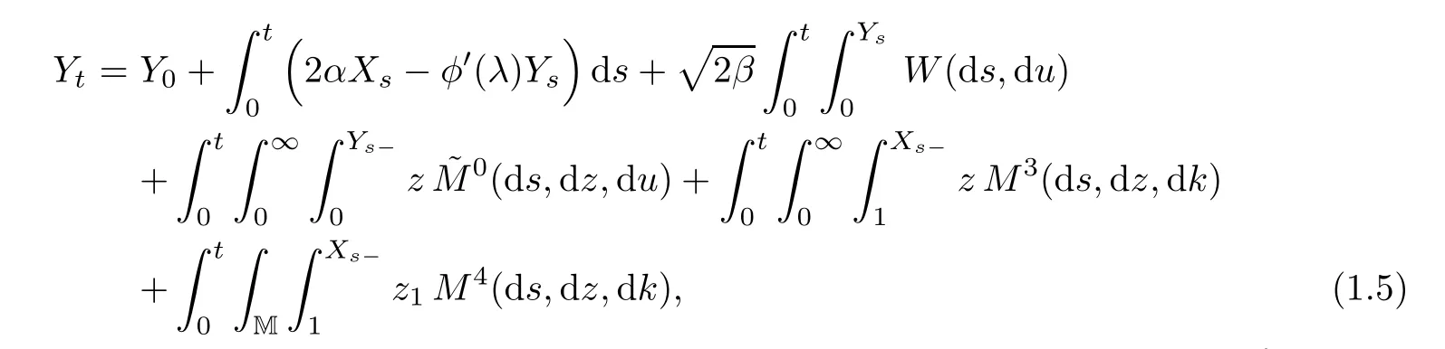
Here M=R+×N,M3(ds,dz,dk)is a Poisson random measure on(0,∞)2×{N{0}}with intensity measure dsze?λzm(dz)?(dk),M4(ds,dz,dk)is a Poisson random measure on(0,∞)×M×{N{0}}with intensity measure φ′(λ)dsηz2(dz1)pz2?(dz2)?(dk),and one can see the speci fic de finitions of two distributions(ηk)k∈Nand(pk)k∈Nin[9,p.1127],so we omit them here.The authors prove that,for any y≥0,{Yt:t≥0}is a weak solution of(1.4)with initial value Y0=y if X0is Poisson distributed with parameter λy.Moreover,(1.5)–(1.6)includes the proli fic skeleton decomposition when λ=λ?;see[2]for the properties of this special decomposition.We refer to[10]for a similar construction of(1.5)–(1.6)in the setting of superprocesses.

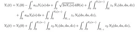
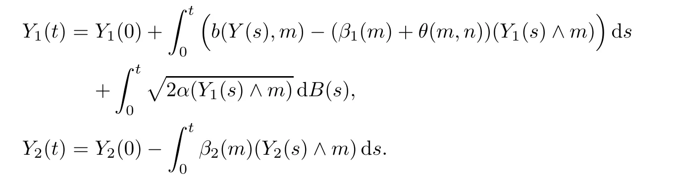
Inspired by the formulations(1.5)–(1.6),the first objective of this paper is to construct a two-dimensional branching Markov process{(Y1(t),Y2(t)):t≥0}taking values in M obtained as a unique strong solution to a more generalized stochastic equation system than(1.5)–(1.6);the process is called the continuous time mixed state branching process(MSB-process).The speci fic form of the stochastic equation system is as follows:

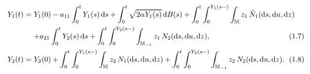
Here,a21,α≥0,a11∈R,M?1=R+×N?1,N?1=N∪{?1},B is a standard Brownian motion,N1and N2are two Poisson random measures with intensity measures dsn1(dz)du and dsn2(dz)du,respectively,and n1and n2are two Lvy measures satisfying some moment conditions.Intuitively,there exist interactions between{Y1(t):t≥0}and{Y2(t):t≥0},therefore(1.7)–(1.8)obviously generalize(1.5)–(1.6).We mention that the Brownian motion B in(1.7)can be replaced by a space-time white noise W and the process has the same law for any fixed initial value.

In the literature on the theory of branching processes,the rescaling approach plays a valuable role in establishing the connection among those branching processes;this leads to the second purpose of this paper,and the establishment of two results.First,for a sequence of GW-processes{Xk(n):n≥0}k≥1and a positive sequence{γk}k≥1,we show that on proper conditions,{Xk():t≥0}converges as k→∞to a DB-process in distribution,wheredenotes the integral part of x.Second,for a sequence of two-type GW-processes{(Yk,1(n),Yk,2(n)):n∈N}k≥1,we prove that{(k?1Yk,1(),Yk,2()):t≥0}converges in distribution to a MSB-process under parallel conditions.The two limit theorems above are mainly inspired by[22,23,27].

The existence of the stationary distribution and the ergodic rates are both important topics in the theory of Markov processes.Demonstration of a necessary and sufficient condition for the existence of the stationary distribution of one-dimensional CBI-processes was initiated by[31];see also[23]for a proof.The sufficient condition for the multi-type case can be found in[20].The strong Feller property and exponential ergodicity of such processes in the total variation distance were given in[24]by a coupling of CBI-processes constructed by the stochastic equation driven by time-space noises and Poisson random measures;see also[25].In a recent work,[26]considered the ergodicities and exponential ergodicities in Wasserstein and total variation distances of Dawson-Watanabe superprocesses with or without immigration;this clearly includes the multi-type CBI-process case.After constructing the MSB-processes,we also want to study the ergodic theory of such processes and prove the exponential ergodicity in the L1-Wasserstein distance by establishing upper bound estimates for the variations of the transition probabilities;this is inspired by similar results on measure-valued branching processes in[26].Moreover,by adding the immigration structures,we give a sufficient and necessary condition for the existence of the stationary distribution of MSB-processes with immigration(MSBI-processes).

The remainder of this paper is organized as follows:in Section 2,we prove a weak convergence theorem from GW-processes to DB-processes.In Section 3,we obtain the MSB-process arising in a limit theorem of rescaled two-type GW-processes.In Section 4,we provide another construction of MSB-processes by stochastic equation systems.The analysis of distributions of jumps is given in Section 5.In Section 6,we study both the estimates for the variations and the exponential ergodicity in the L1-Wasserstein distance W1for the transition semigroup of such processes.Finally,we prove the existence of the stationary distribution of such processes with immigration in Section 7.

2 The Construction of DB-processes

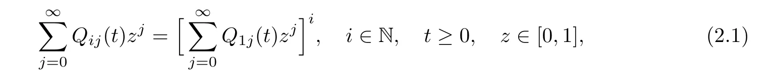
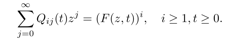
Let{pj:j∈N}be a probability distribution on N,and denote the generating function by g(z)=on|z|≤1.Let u(z)=a(g(z)?z)for some a>0.A Markov process{Xt:t≥0}with state space N is called a DB-process with branching rate a>0 and offspring distribution{pj:j∈N}if its transition probabilities Qij(t)satisfy

which implies the branching property of the process.Denote F(z,t)=Clearly,F=(F(·,t):t≥0)satis fies the semigroup property F(·,t+s)=F(F(·,t),s)for t,s≥0 and is the unique solution of the following differential equation:

We call F the compound semigroup for the DB-process,and refer to[1,p.106-107]for more details.

We now provide a sufficient condition for the weak convergence of GW-processes to the DB-process.Assume that there exists a sequence of GW-processes{Xk(n):n≥0}k≥1with parameters{gk}k≥1,and let{γk}k≥1be a sequence of positive numbers.Denote the n-step transition probability for{Xk(n):n≥1}by,and letx」be the integral part of x.One can see that

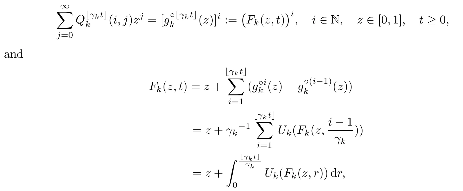
where g°n(z)is de fined by g°n(z)=g(g°(n?1)(z)),successively with g°0(z)=z and Uk(z)=γk(gk(z)?z),0≤z≤1.For convenience,we formulate the following conditions:

(A)γk→∞as k→∞.

(B)The sequence Uk(z)is uniformly Lipschitz on[0,1],and converges to a continuous function u(z)as k→∞.

Proposition 2.1(i)Suppose that(A,B)hold.Then the limit function of sequence{Uk(z)}k≥1has representation u(z)=a(g(z)?z)as k→∞for all 0≤z≤1,where a is a strictly positive constant,g(z)is a generation function and g′(1?)<∞.

(ii)For any given u(z)=a(g(z)?z),there exists a sequence of{Uk}k≥1such that(A,B)hold with Uk(z)→u(z).

Proof(i)The desired result is a corollary of Proposition 3.1(i),to be demonstrated later.Indeed,it suffices to consider the offspring distribution corresponding to two-type GW-processes cases satisfying vk({i,·})≡0 for all i≥1.

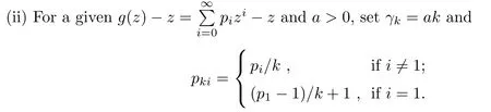
De fining Uk(z)=,it is not hard to see that Uksatis fies condition(B),and converges to u(z)for all z∈[0,1].

Lemma 2.2Suppose that(A,B)hold.Then there are constants λ,N≥0 such that Fk(z,t)∈for every t≥0,z∈[0,1]and k≥N.

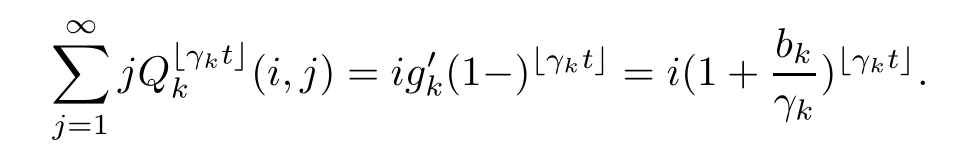
ProofLet bk:=γk((1?)?1).Under condition(B),there exists λ≥0 such that 2|bk|≤λ for all k≥1.It is not hard to obtain that

Since γk→∞as k→∞,there is a N≥1 such that,for all k≥N,

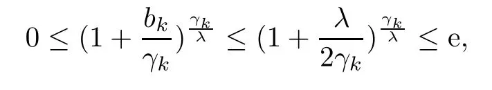
so for t≥0 and k≥N,

We get the desired result by Jensen’s inequality.

Lemma 2.3Suppose that(A,B)hold.For any c>0,we have Fk(z,t)→some F(z,t)uniformly on[0,e?c]×[0,c]as k→∞,and the limit function solves(2.2).

ProofWe may rewrite

By Proposition 2.1 and Lemma 2.2,for ε∈(0,1],we can take N≥1 large enough such that

Denote the last term on the right hand of equation(2.3)by εk(t,z).Then

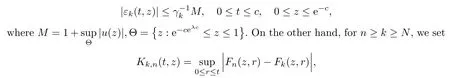
and it follows that

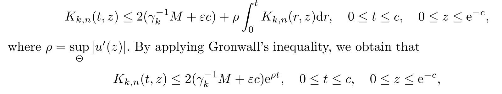
from which it follows that Fk(z,t)→some F(z,t),and the limit function satis fies(2.2).

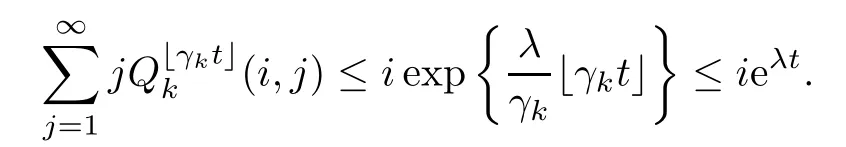
By(2.1),we see that the transition probabilities Q={Qij(t):i,j∈N,t≥0}of the DB-process{Xt:t≥0}can be determined by

Based on Proposition 2.1 and Lemma 2.3,by similar arguments as to those of Theorem 2.9 in[25],it is not hard to see that the transition probability Q of{Xt:t≥0}is a limit of a sequence of transition probabilities{(i,j):i,j∈N,t≥0}k≥1associated with GW-processes in the sense of weak convergence under conditions(A,B);this indeed implies another construction of DB-processes by a rescaling approach.

3 The Construction of MSB-processes

For a two-type GW-process{Y(n)=(Y1(n),Y2(n)):n∈N},we de fine two corresponding generation functions for i=(i1,i2)∈N2and s1,s2∈[0,1]:

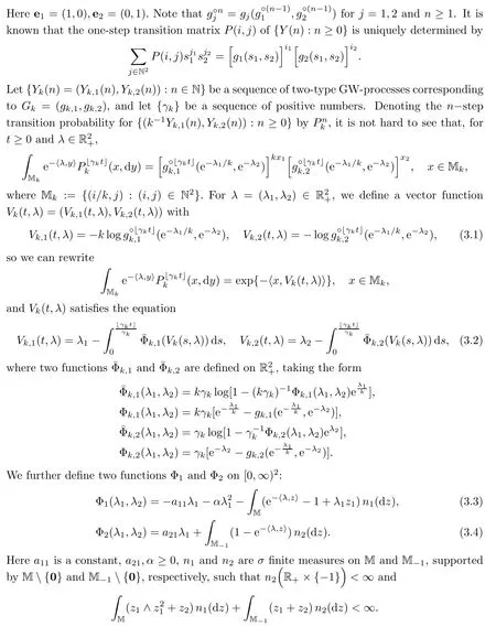
For convenience,let us consider the following conditions:(A)γk→∞.

(C)The sequence{Φk,1(λ1,λ2)}k≥1is uniformly Lipschitz in(λ1,λ2)on each bounded rectangle,and converges to a continuous function as k→∞.

(D)The sequence{eλ2Φk,2(λ1,λ2)}k≥1is uniformly Lipschitz in(λ1,λ2)on each bounded rectangle,and converges to a continuous function as k→∞.

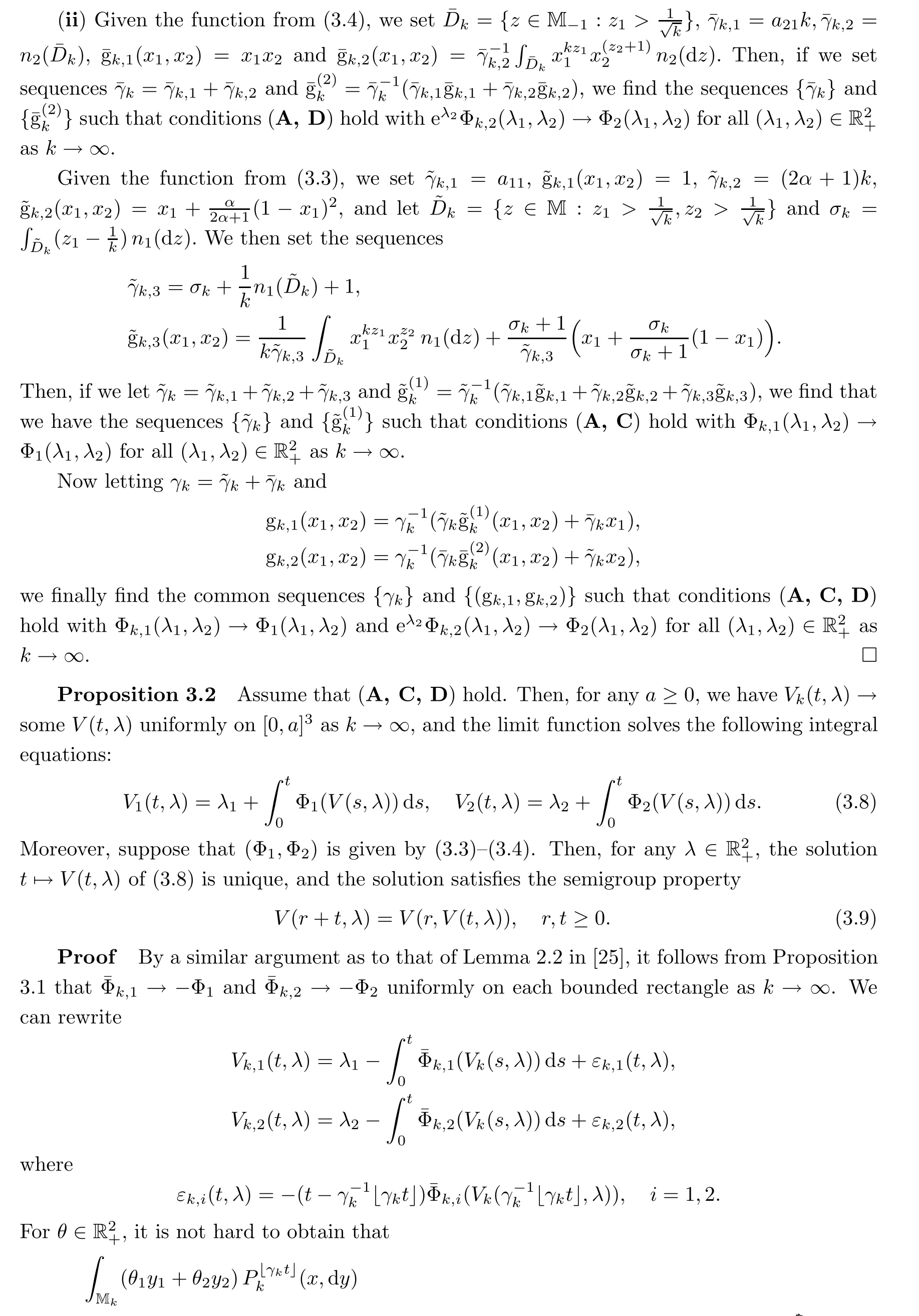
By a modi fication of the proof of Lemma 2.6 and Theorem 2.7 in[25],we get(3.8).For given(Φ1,Φ2)by(3.3)–(3.4),it follows from Proposition 3.1(ii)that there is a sequence{Φk,1,Φk,2}satisfying(A,C,D),so if we let a sequence{Vk}be given by(3.1)and(3.2),the existence of the solution is immediate.The uniqueness of the solution follows by Gronwall’s inequality,and the semigroup property follows from the uniqueness of the solution.

Proposition 3.3Suppose(Φ1,Φ2)are given by(3.3)–(3.4).For any λ∈,let t→V(t,λ)be the unique positive solution to(3.8).Then we can de fine a transition semigroup(Pt)t≥0by

ProofGiven(Φ1,Φ2)by(3.3)–(3.4),by Proposition 3.1,there is a sequence(Φk,1,Φk,2)satisfying(A,C,D).By Proposition 3.2,for any a≥0 we have Vk(t,λ)→V(t,λ)uniformly on[0,a]3as k→∞.Take xk∈Mksatisfying xk→x as k→∞.Then,by a continuity theorem(see,e.g.,Theorem 1.18 in[23]),(3.10)de fines a probability measure on M and(xk,·)=Pt(x,·)by weak convergence.The semigroup property of the family of(Pt)t≥0follows from(3.9)and(3.10).

De finitionA Markov process{Y(t)=(Y1(t),Y2(t)):t≥0}is called a MSB-process with state space M if it has the transition semigroup(Pt)t≥0in(3.10).

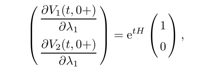
Proposition 3.4Let(Pt)t≥0be the transition semigroup de fined by(3.10).Then we have

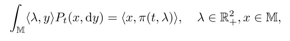
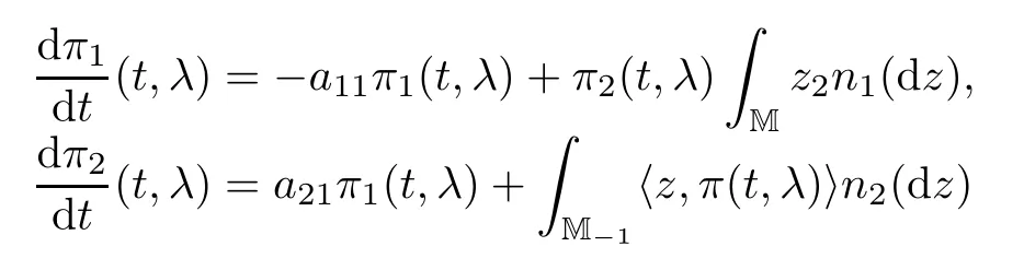
with initial condition π(0,λ)=λ.

ProofOne can see that V(t,0+)=0 for t≥0.By differentiating both sides of(3.10)with respect to λ1and λ2,we have

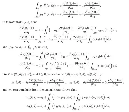
and the desired assertion follows.

By a modi fication of the proof of Theorem 2.11 in[25],one can see that the semigroup de fined by(3.10)is a Feller semigroup.Then the MSB-process has a c`adl`ag realization.Moreover,the MSB-process can also be characterized in terms of the martingale problem described as follows(see Corollary 4.4 below for the proof):for f∈C2(M),let L be an operator acting on C2(M)de fined by

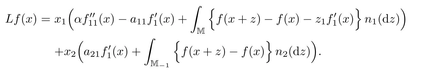
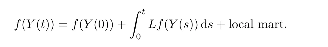
Suppose that{(Y1(t),Y2(t)):t≥0}is a non-negative cdlg process withE[Yi(0)]<∞,i=1,2.Then{(Y1(t),Y2(t)):t≥0}is a MSB-process with transition semigroup(Pt)t≥0if and only if,for every f∈C2(M),

Theorem 3.5Assume that(A,C,D)hold,and that(Yk,1(0)/k,Yk,2(0))converges to(Y1(0),Y2(0))in distribution.Then

in distribution on D([0,∞),M)as k→∞.

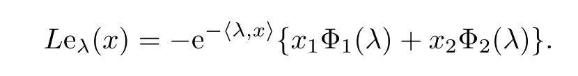
ProofLet L be the generator of the MSB-process.For λ=(λ1,λ2)?0,x∈M,set eλ(x)=e?〈λ,x〉.We have

Denote by D1the linear hull of{eλ,λ?0}.Then D1is an algebra which strongly separates the points of M.Let C0(M)be the space of the continuous function on M vanishing at in finity.By the Stone-Weierstrass theorem,D1is dense in C0(M)for the supremum norm.Noting that D1is invariant under Ptby(3.10),it follows from Proposition 3.3 in Chapter I of[8]that D1is the core of L.Note that{Yk,1(n)/k,Yk,2(n):n≥0}is a Markov chain with state space Mk,and the one-step transition probability is determined by

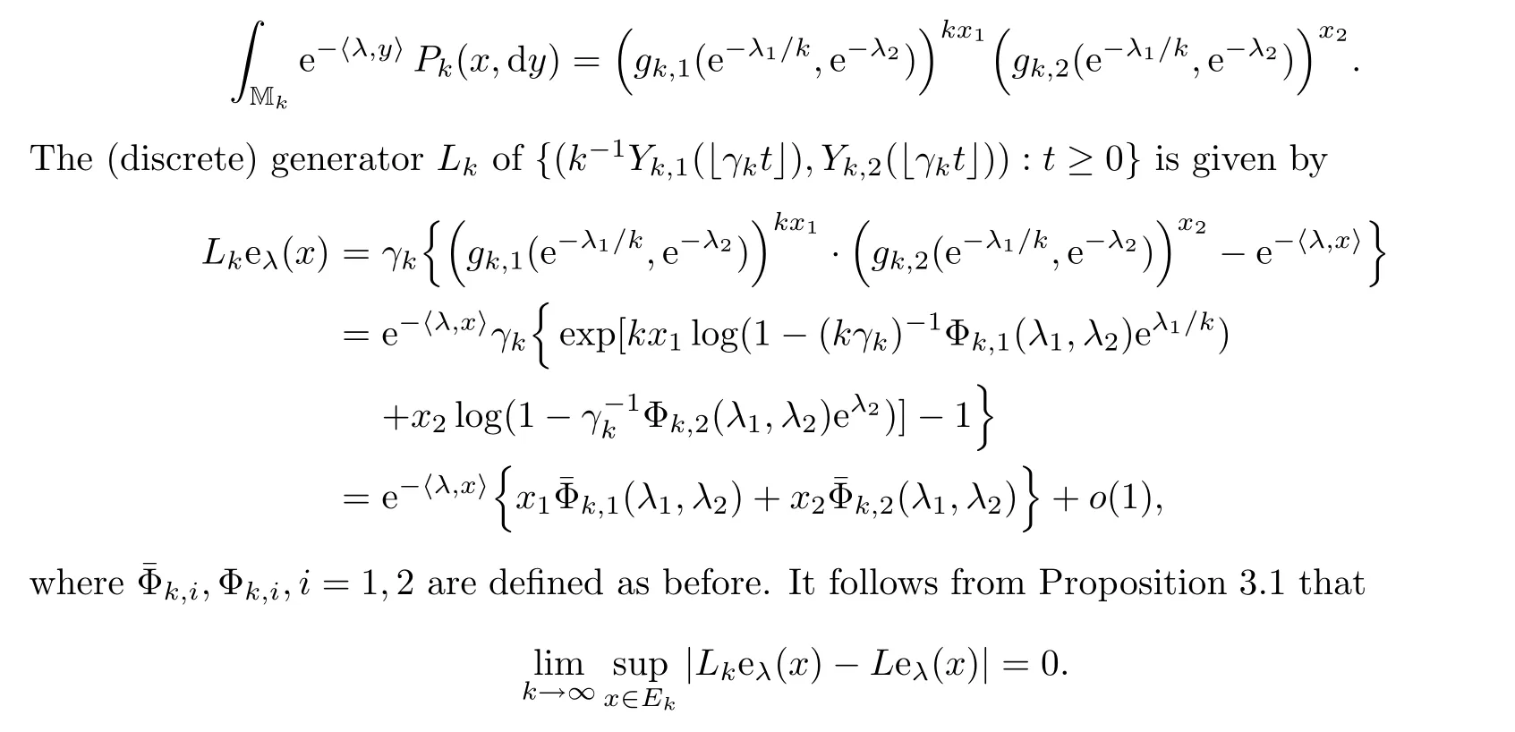
From Corollary 8.9 in Chapter 4 of[8],we prove the desired result.

Theorem 3.6Suppose that{(Y1(t),Y2(t)):t≥0}is any MSB-process with(Φ1,Φ2).Then,there exist a sequence of positive numbers{γk}and a sequence of two-type GW-processes{(Yk,1(n),Yk,2(n)):n∈N}with generation functions(gk,1,gk,2)such that the sequence{(k?1Yk,1(),Yk,2()):t≥0}converges in distribution on D([0,∞),M)to the process{(Y1(t),Y2(t)):t≥0}as k→∞.

ProofBy Proposition 3.1,there exist{γk},{(gk,1,gk,2)}such that conditions(A,C,D)hold.The desired result follows from Theorem 3.5.

4 The Construction of MSB-processes by Stochastic Equations

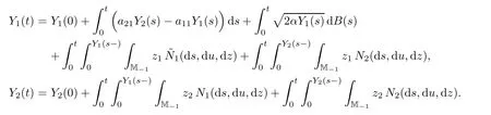
Let(?,F,Ft,P)be a complete filtered probability space satisfying the usual hypotheses,let{B(t)}be a standard Brownian motion,let{N1(ds,du,dz)}be a Poisson random measure on(0,∞)2×M with intensity dsdun1(dz),and let{N2(ds,du,dz)}be a Poissonrandom measure on(0,∞)2×M?1with intensity dsdun2(dz),z=(z1,z2).Suppose that B,N1,N2are independent of each other.Let us recall the stochastic integral equation system(1.7)–(1.8)

Proposition 4.1Suppose that{Y(t)}satis fies(1.7)–(1.8)andP{Y(0)≥0}=1.ThenP{Y(t)≥0,?t≥0}=1.

ProofBy equation(1.8),if Y2(0)≥0,it is not hard to see that,for all t≥0,Y2(t)≥0.Now suppose that there exists ε>0 such that τ:=inf{t>0,Y1(t)≤?ε}<∞with strictly positive probability.Then there exists t0>0,Y1(t0)=0,and on the time interval[t0,τ],tY1(t)is a strictly negative continuous function.Hence there are some t1∈[t0,τ]and δ>0 such that,for all s∈[t0,t1],?a11Y1(s)+a21Y2(s)≥δ.Then

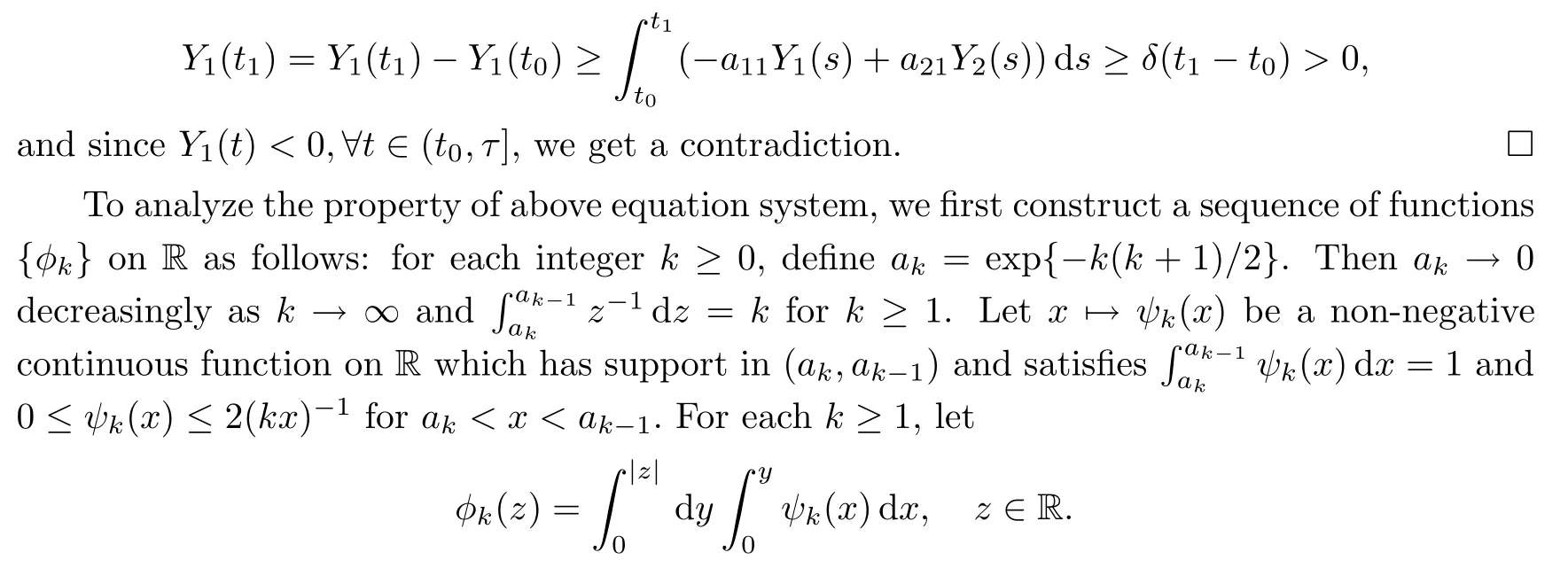
Moreover,for function f on R,we denote

Theorem 4.2The pathwise uniqueness for(1.7)–(1.8)holds.

ProofSuppose that{Y(t)}and{Y′(t)}are two solutions of(1.7)–(1.8).Let ζi(t)=Yi(t)?(t),i=1,2 for t≥0.We have

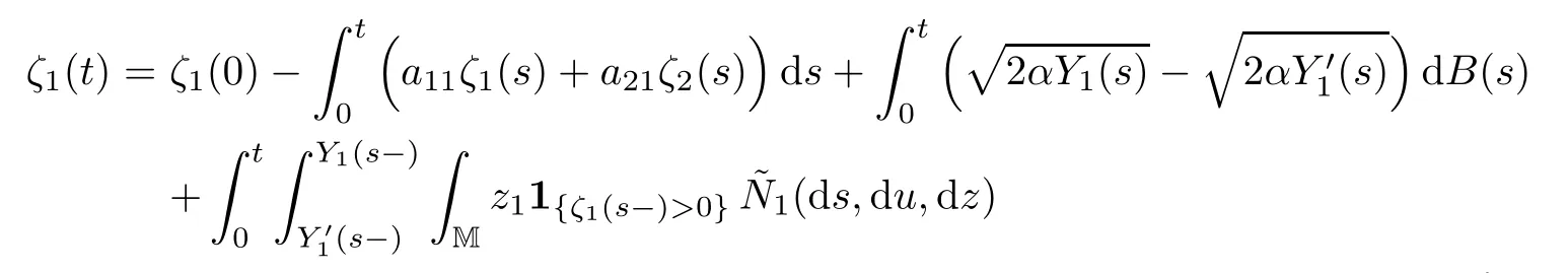
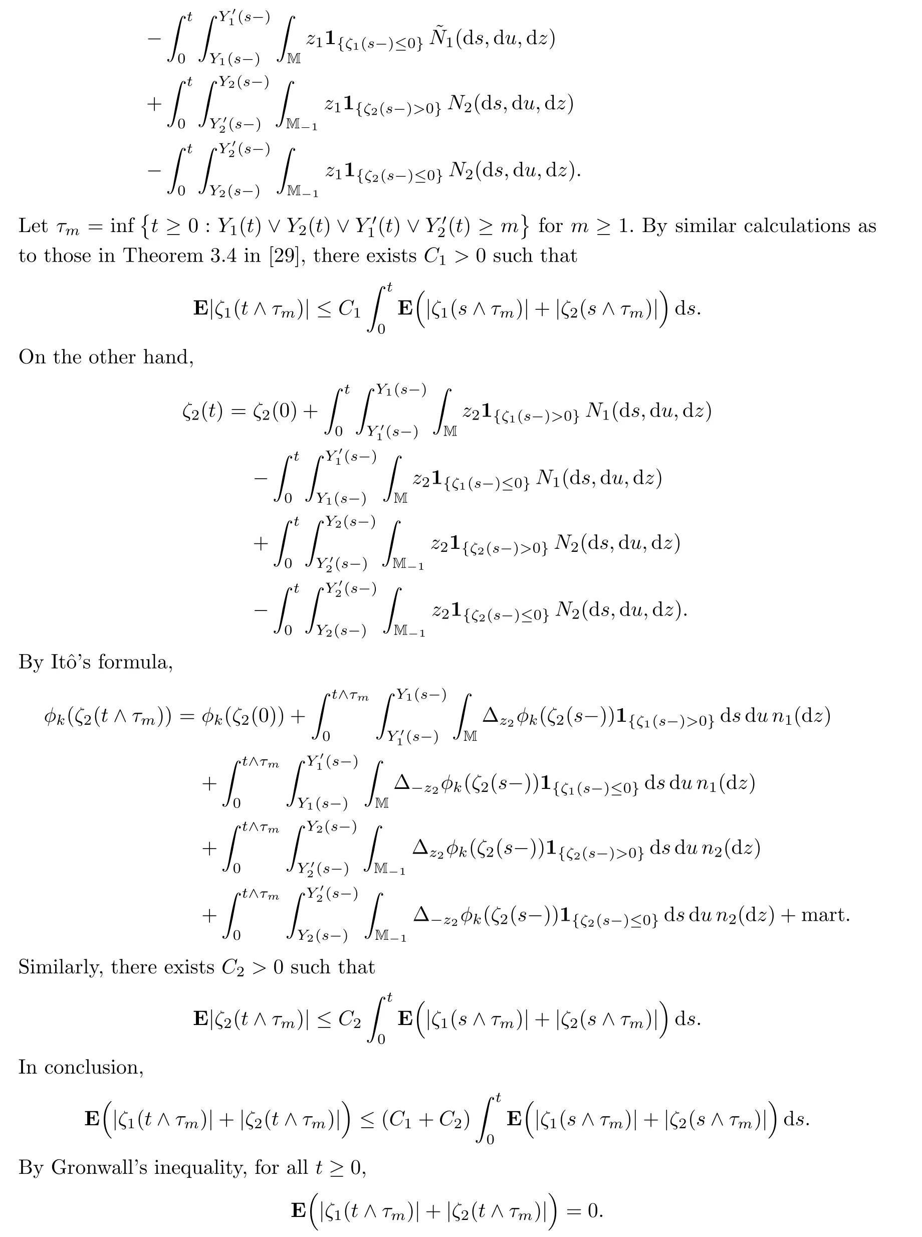
Since{Y(t)}and{Y′(t)}have c`adl`ag sample paths,we conclude thatP{Y(t)=Y′(t),?t≥0}=1 as m→∞.

Theorem 4.3There is a unique non-negative strong solution to(1.7)–(1.8).

ProofSince ν1is supported on M{0},we can rewrite(1.7)–(1.8)as

For any fixed n≥1,let Vn={z∈M?1:‖z‖≥1/n},so n1(Vn)+n2(Vn)<∞.For m≥1 and x∈M,de fine

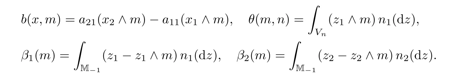
By the results for continuous-type stochastic equations in[15,p.169],one can show that there is a non-negative weak solution to the following stochastic equation system:

The pathwise uniqueness holds for the above system of equations by similar arguments as to those in Theorem 4.2.Then it has a unique strong solution.By similar arguments as to those in the proof of Proposition 2.2 in[13],we can get a pathwise unique non-negative strong solution{Ym,n(t):t≥0}to(4.1)–(4.2)as follows:

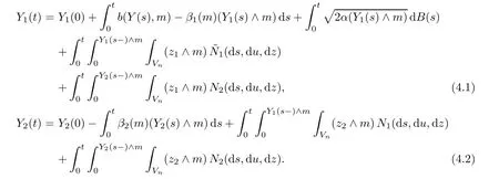
As in the proof of Lemma 4.3 in[13],one can see that the sequence{Ym,n(t):t≥0},n=1,2,···is tight in D([0,∞),M).Following the proof of Theorem 4.4 in[13],it is easy to show that any weak limit point{Ym(t):t≥0}of the sequence is a non-negative weak solution to

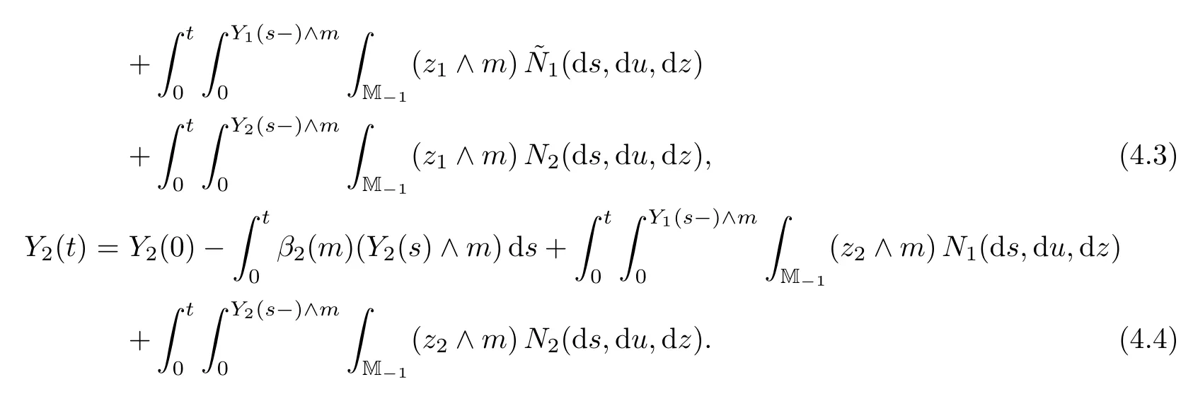
By Theorem 4.2,the pathwise uniqueness holds for(4.3)–(4.4),so the system of equations has a unique strong solution.Finally,the desired result follows from a modi fication of the proof of Proposition 2.4 in[13].

Corollary 4.4A c`adl`ag non-negative process is a MSB-process with transition semigroup(Pt)t≥0de fined by(3.8)and(3.10)if and only if it is a weak solution of(1.7)–(1.8).

ProofSuppose that{(Y1(t),Y2(t))}t≥0is a weak solution of(1.7)–(1.8).By It?o’s formula,one can see that{(Y1(t),Y2(t))}t≥0solves the martingale problem associated with the generator L.By the arguments in Section 3,we infer that{(Y1(t),Y2(t))}t≥0is a MSB-process with a transition semigroup(Pt)t≥0de fined by(3.8)and(3.10).Conversely,suppose that{(Y1(t),Y2(t))}t≥0is a c`adl`ag realization of the MSB-process with transition semigroup(Pt)t≥0de fined by(3.8)and(3.10).Then the distributions of{(Y1(t),Y2(t))}t≥0on D([0,∞),M)can be characterized uniquely by the martingale problem.By a standard stopping time argument,we have

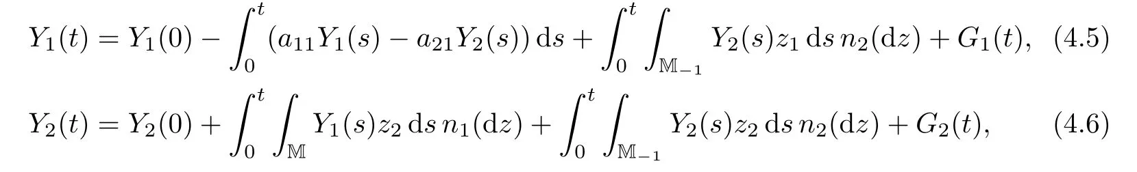
where G1(t)and G2(t)are two square-integrable local martingales.Let N0(ds,dz)be the optimal random measure on[0,∞)×M?1de fined by

It follows from[7,p.376]that

dC1(t)=2αY1(t)dt and dC2(t)=0.Then we obtain the equation(1.7)–(1.8)on an extension of the probability space by applying martingale representation theorems;see,e.g.,[15,p.93,p.84].This completes the proof.

5 The Distribution of Local Jumps

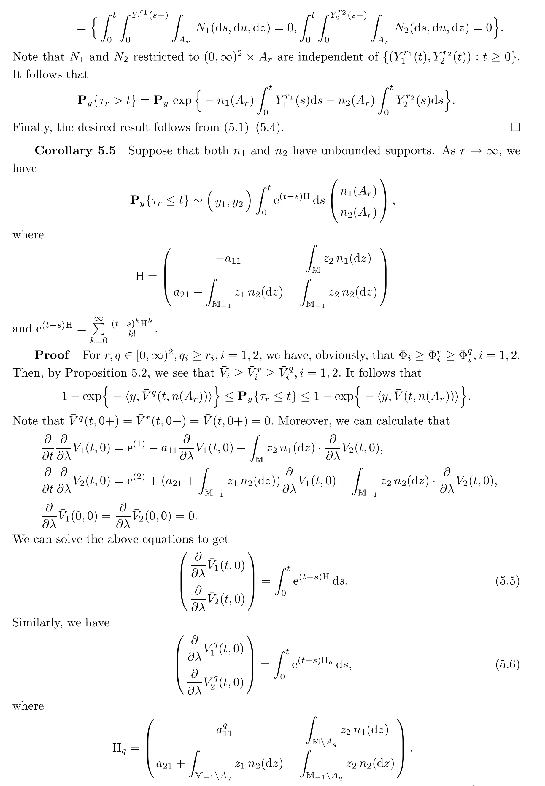
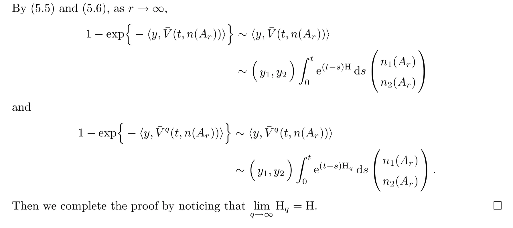
For any initial time r≥0,let Y=(?,F,Fr,t,Y(t),Pr,y:t≥r,y≥0)be a Hunt realization of the MSB-process with transition semigroup(Pt)t≥0de fined by(3.8)and(3.10).Here,{Pr,y:y≥0}is a family of probability measures on(?,F,Fr,t)satisfyingPr,y{Y(r)=y}=1 for all y≥0.For any t≥r≥0 and λ∈[0,∞)2,we have

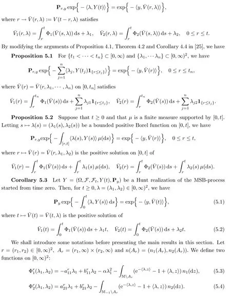
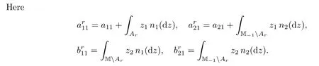
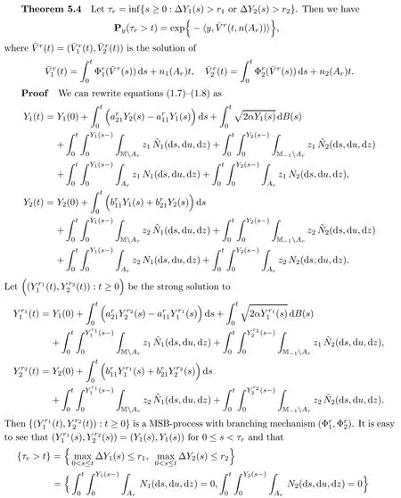
The following theorem gives a characterization of the distribution of the local maximal jump of the MSB-process:

6 Exponential Ergodicity in Wasserstein Distances

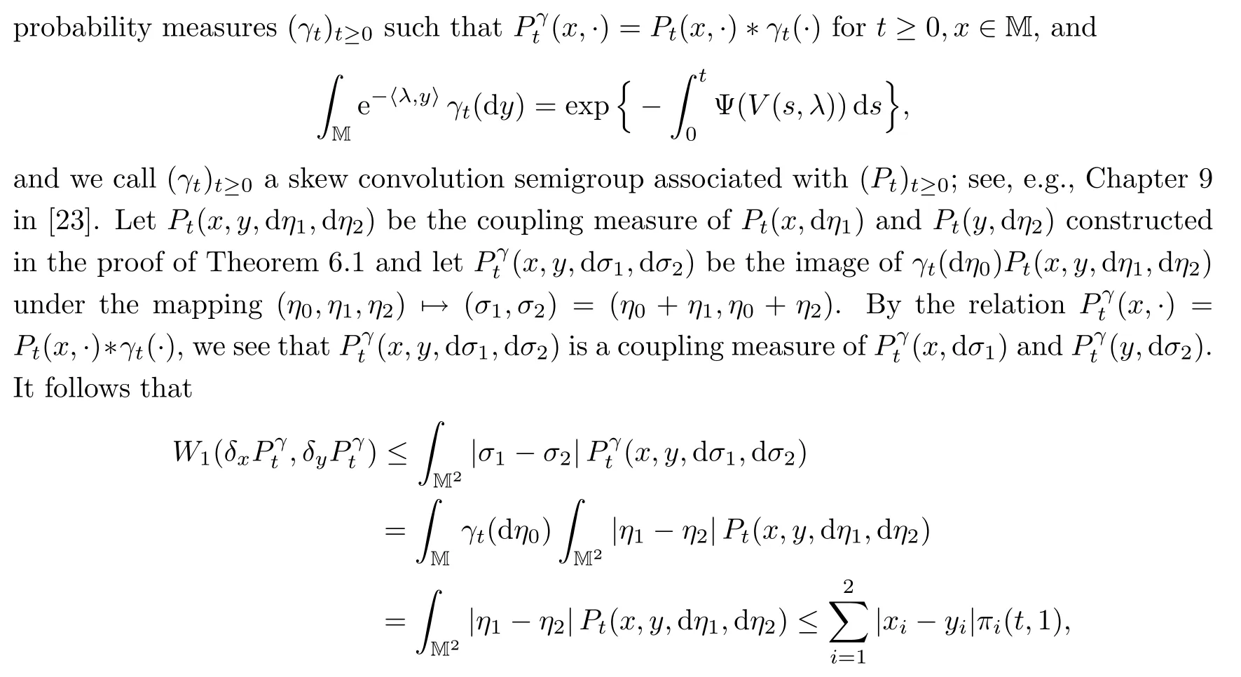
In order to present our results in this section,we first introduce some notations.Given two probability measuresμand ν on M,the standard Lp-Wasserstein distance Wpfor all p≥1 is given by

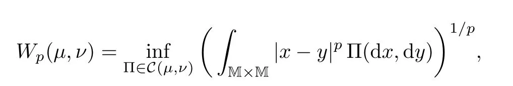
where|·|denotes the Euclidean norm and C(μ,ν)stands for the set of all coupling measures ofμand ν,i.e.,C(μ,ν)is the collection of measures on M×M havingμand ν as marginals.Denoting Pp(M)as the set of probability measures having a finite moment of order p,it is known that(Pp(M),Wp)becomes a Polish space.

The next theorem gives the upper and lower bounds for the variations in the L1-Wasserstein distance W1of the transition probabilities of the MSB-process started from two different initial states.

Theorem 6.1Let(Pt)t≥0be the transition semigroup de fined by(3.10).Then for all x,y∈M and t≥0,we have

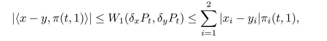
where δxPt(·):=Pt(x,·)and π(t,1)is de fined as in Proposition 3.4 with λ=(1,1).

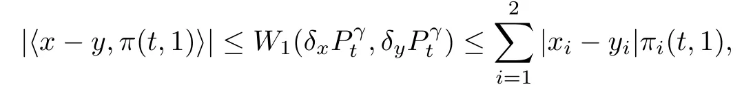
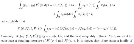
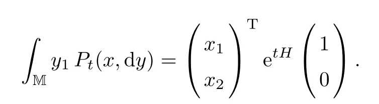
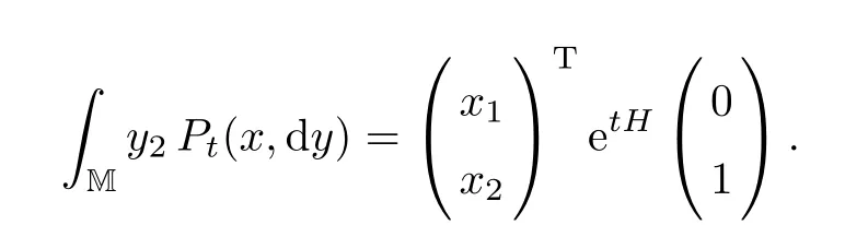
ProofThe proof is based on the same idea as that of Theorem 2.2 in[26].By Proposition 3.4,we see thatRM(y1+y2)Pt(x,dy)=〈x,π(t,1)〉.It follows from Theorem 5.10 in[4]that

Similarly,W1(δxPt,δyPt)≥〈y?x,π(t,1)〉.Then the first inequality follows.On the other hand,for x,y∈M,let(x?y)±:=((x1?y1)±,(x2?y2)±),and x∧y:=x?(x?y)+=y?(x?y)?.Let Pt(x,y,dη1,dη2)be the image of the product measure

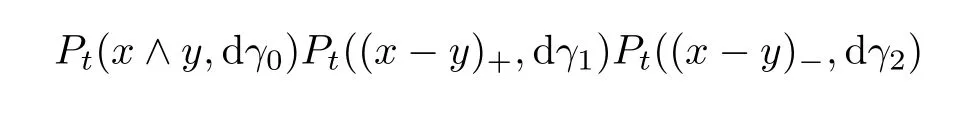
under the mapping(γ0,γ1,γ2)(η1,η2):=(γ0+γ1,γ0+γ2).It is not hard to see that Pt(x,y,dη1,dη2)is a coupling of Pt(x,dη1)and Pt(y,dη2).Then

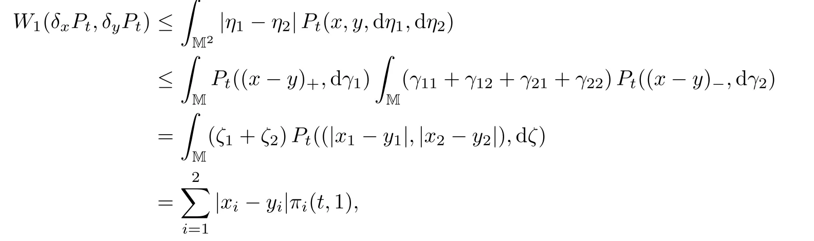
where we have used the branching property Pt(a,·)?Pt(b,·)=Pt(a+b,·)for all a,b∈M,t≥0 in the third row.Therefore the proof is finished.

Based on Theorem 6.1,we can establish the exponential ergodicity with respect to W1.Recalling that a 2×2 matrix H=[Hij]2×2in Corollary 5.5 is de fined as

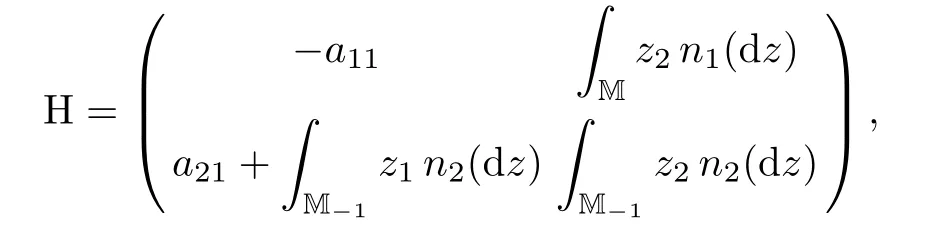
we have the following result:

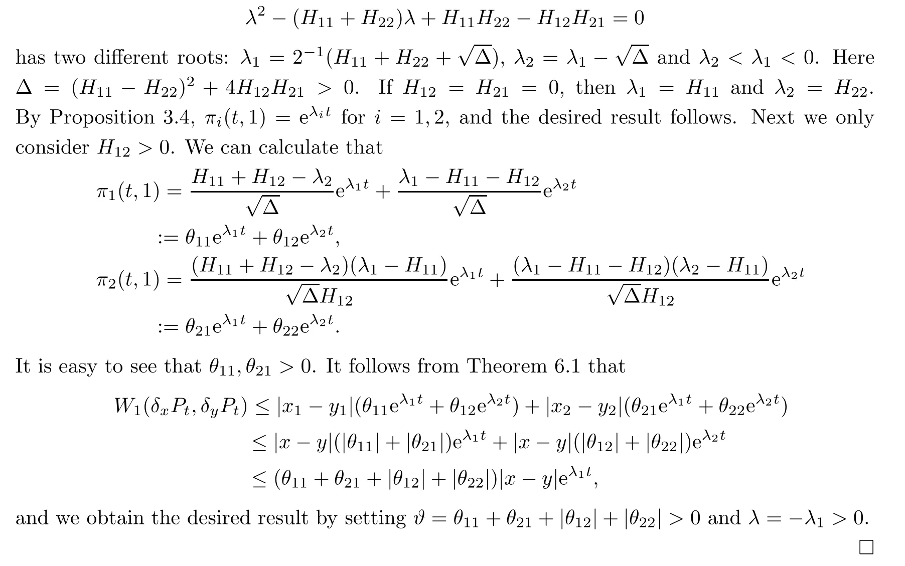
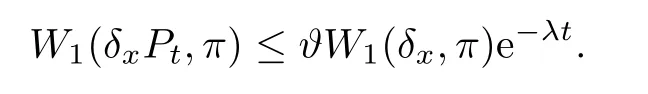
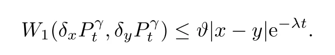
Theorem 6.2Assume that H11H22?H12H21>0 and H11+H22<0.Then there exist λ,?>0 such that,for any t≥0 and x,y∈M,

ProofBy assumption,it is easy to see that

Corollary 6.3Assume that the conditions of Theorem 6.2 hold.Then there exist a unique π∈P1(M)and ?,λ>0 such that,for any x∈M and t≥0,

ProofBy Theorem 7.5 below,there exists a unique invariant measure.Arguing similarly as to the proof of Theorem 3.2 in[12],one can see that π∈P1(M),and the desired assertion is easily obtained by Theorem 6.2.

7 MSBI-processes

Suppose that Φ1,Φ2are two functions on[0,∞)2de fined as in(3.3)–(3.4),and that there exists function Ψ on[0,∞)2de fined by

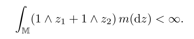
where b>0 and m is a σ-fi nite measure on M supported by M{0}such that

A Markov process{Z(t)=(Z1(t),Z2(t)):t≥0}is called a MSBI-process on M if it has a transition semigroup()t≥0uniquely determined by

where V(t,λ)=(V1(t,λ),V2(t,λ))takes values onand satis fies(3.8).One can see that the semigroup de fined by(7.2)is a Feller semigroup,so the MSBI-process has a cdlg realization.We can also establish a similar result as to that of Theorem 6.1 for MSBI-processes;indeed,we have the following:

Theorem 7.1Let()t≥0be the transition semigroup de fined by(7.2).Assume that<∞.Then,for t≥0 and x,y∈M,we have

where π(t,1)is de fined as in Proposition 3.4 with λ=(1,1).

ProofThe proof is based on the same idea as that of Theorem 4.1 in[26].One can see that

where the last inequality follows from Theorem 6.1.

By a similar argument as to that of Theorem 6.2,we have

Theorem 7.2Assume that H11H22?H12H21>0 and H11+H22<0.Then,there exist λ,?>0 such that,for any t≥0 and x,y∈M,

7.1 The construction of MSBI-processes by stochastic equations

We now give a construction of MSBI-processes by stochastic equations.Let us consider the stochastic equation system

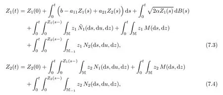
where b≥0,M(ds,dz)is a Poisson random measure on[0,∞)×M with intensity measure dsm(dz),and the other coefficients are the same as in Section 4.Furthermore,we assume that those random elements are independent of each other.By a modi fication of the proof of Section 4,as well as that in[28],we see that(7.3)–(7.4)has a unique strong solution and is a MSBI-process with branching mechanism(Φ1,Φ2)de fined by(3.3)–(3.4)and an immigration mechanism Ψ de fined by(7.1).

7.2 Stationary distribution

In order to characterize the stationary distribution of MSBI-processes,we need to estimate the upper and lower bounds of|V(t,λ)|for t>0,λ∈;this will play an important role in the sequel.

Lemma 7.3Let(Yt)t≥0be a MSB-process with semigroup(Pt)t≥0satisfying(3.10).Let H=[Hij]2×2be a 2×2 matrix de fined as in Corollary 5.5.Suppose that all the eigenvalues of H have strictly negative real parts.Then there exist some strictly positive constants c1(λ)and c2where c1depends on λ such that

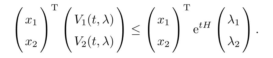
ProofWe follow the same calculations as those in Proposition 3.4 to see that

and so

Similarly,

By Jensen’s inequality,we deduce that,for all x=(x1,x2)∈M,

Since all the eigenvalues of H have strictly negative real parts,there exist some strictly positive c,c2>0 such that,for all t>0,

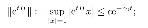
see,e.g.,equation(2.8)in[32],which implies that|V(t,λ)|≤|λ|ce?c2t.We finish the proof by setting c1(λ)=|λ|c.

Lemma 7.4Under the conditions of Lemma 7.3,for every λ∈,there exist two strictly positive constants A(λ)and B(λ)such that

Proof

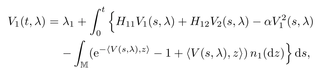
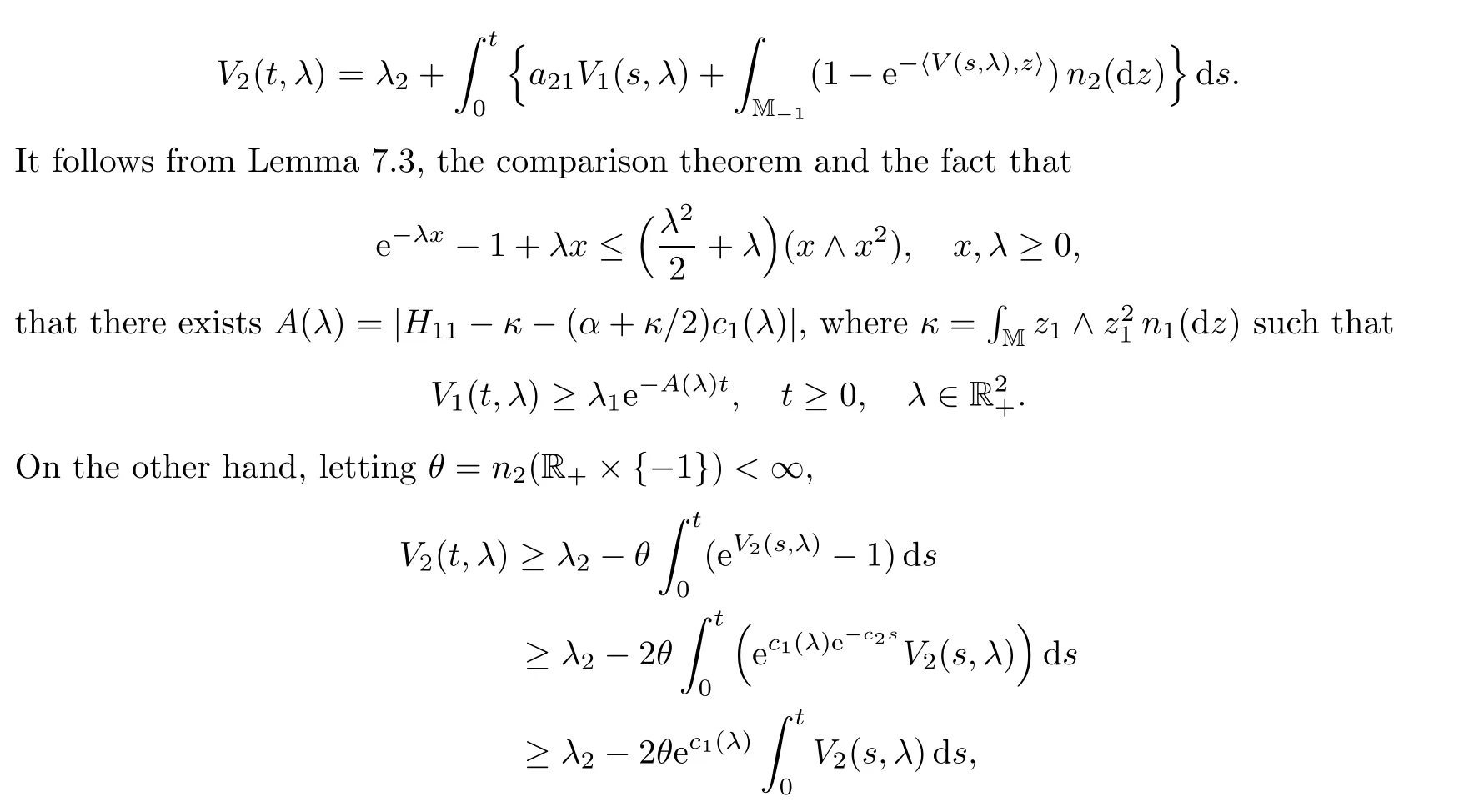
and by the comparison theorem we deduce that V2(t,λ)≥and we obtain the desired result by setting B(λ)=2θec1(λ).

We now give our main result.

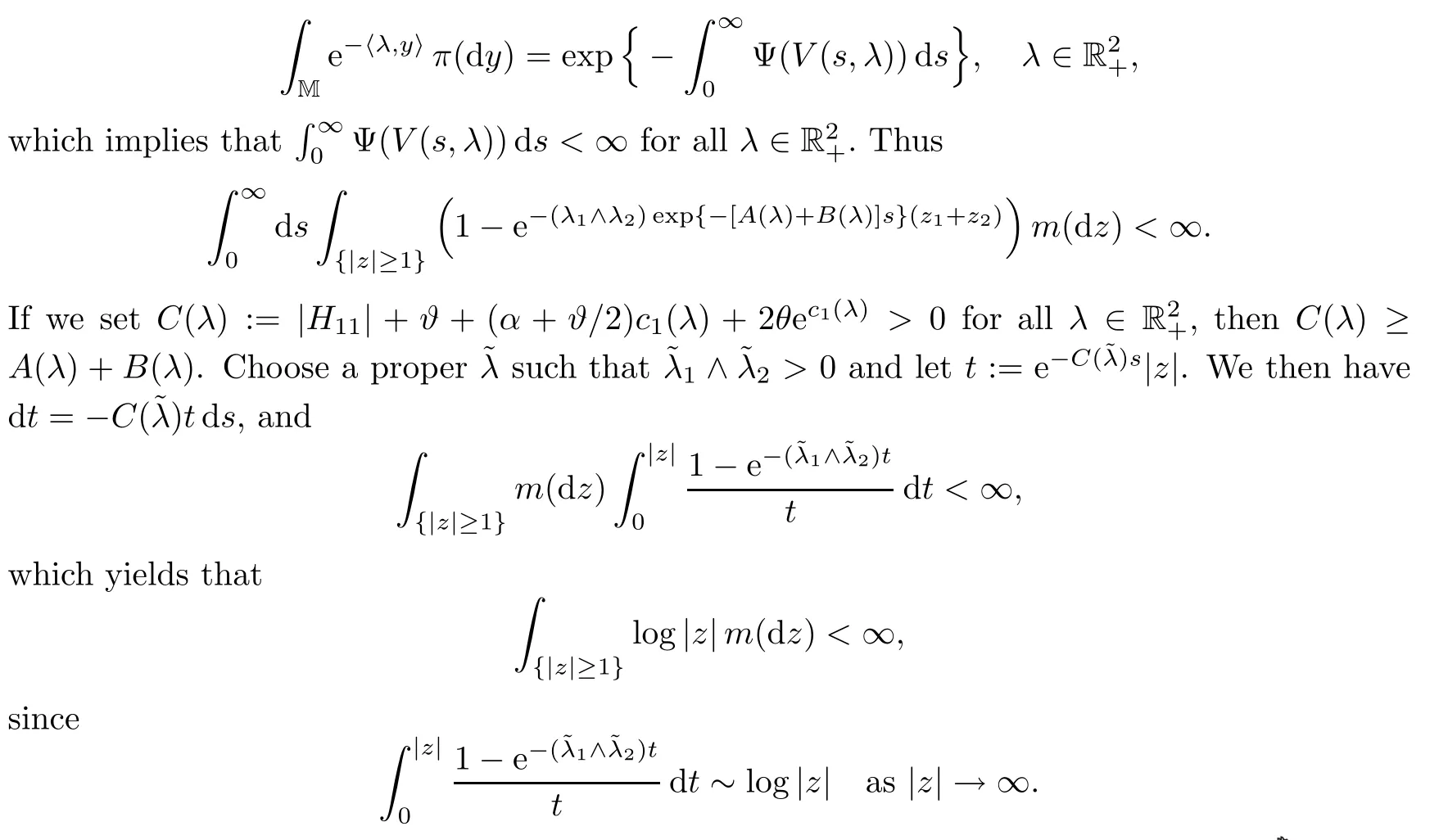
Theorem 7.5Let(Zt)t≥0be a MSBI-process with semigroup()t≥0satisfying(7.2).Suppose that all the eigenvalues of H have strictly negative real parts.Then(x,·)converges to a probability measure π on M as t→∞for all x∈M if and only if

ProofBy Lemma 7.3 we have|V(t,λ)|→0 as t→∞.Supposing that(Zt)t≥0has a stationary distribution π,one can see that

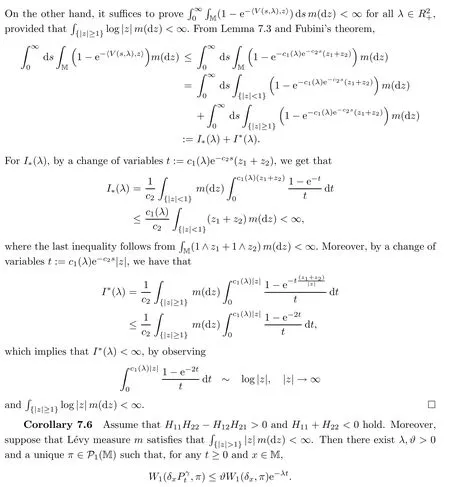
ProofIt follows from Theorem 7.5 and the assumptions that there exists a unique stationary distribution π.We can easily derive thatEx[|Zt|]<∞for all t≥0 and x∈M by the assumption thatR{|z|>1}|z|m(dz)<∞.By a modi fication of the proof of Corollary 6.3,we have that π∈P1(M),and the desired result follows from Theorem 7.2.