A class of two-dimensional rational maps with self-excited and hidden attractors

Li-Ping Zhang(張麗萍) Yang Liu(劉洋) Zhou-Chao Wei(魏周超)Hai-Bo Jiang(姜海波) and Qin-Sheng Bi(畢勤勝)

1Faculty of Civil Engineering and Mechanics,Jiangsu University,Zhenjiang 212013,China

2School of Mathematics and Statistics,Yancheng Teachers University,Yancheng 224002,China

3College of Engineering,Mathematics and Physical Sciences,University of Exeter,Exeter EX4 4QF,UK

4School of Mathematics and Physics,China University of Geosciences,Wuhan 430074,China

Keywords: two-dimensional rational map, hidden attractors, multi-stability, a line of fixed points, chaotic attractor

1. Introduction

Recently,hidden attractor has become an attractive topic for researchers in non-linear sciences, and has been found in many practical systems, such as the Chua system,[1-3]the drilling system,[4]and the automatic control system with piecewise-linear non-linearity.[5]They have been explored intensively in continuous dynamical systems with different structures of equilibria (see Ref. [6]). As it is known, if a dynamical system with a given set of parameters has more than one attractor according to its initial conditions,this phenomenon is called multi-stability. Multi-stability has been studied extensively in the literature since it exists in many areas, such as physics, chemistry, biology and economics (see,e.g.,Refs.[7-11]).

Many researchers have studied the self-excited and hidden attractors in discrete-time maps because of their broad applications (see e.g., Refs. [12-24]). Among these works, a few studies[15-19]have identified the attractors with particular types of fixed points. For example, Jianget al.[15,16]explored the hidden chaotic attractors with no fixed point and a single stable fixed point in a class of two-dimensional and three-dimensional maps, respectively. Jianget al.[17]studied the hidden chaotic attractors in a class of two-dimensional chaotic maps with closed curve fixed points. Luo[19]analyzed the complexity and singularity of a class of discrete systems with infinite-fixed-points by using the local analysis methods.Also,hidden attractors have been found in the non-linear maps in a fractional form.[20-25]In Ref. [20], Ouannaset al.studied a fractional map with no fixed point that exhibits hidden attractors. Hadjabiet al.proposed two new classes of twodimensional fractional maps with closed curve fixed points and studied their dynamics in Ref. [21]. Great efforts[26-30]have also been made for searching and controlling hidden attractors. For example,Dudkowskiet al.[26,27]presented a new method to locate hidden and coexisting attractors in non-linear maps based on the concept of perpetual points. In Ref. [28]Danca and Fe?can used impulsive control to suppress chaos and produced hidden attractors in a one-dimensional discrete supply and demand dynamical system. Then, Danca and Lampart[29]proposed an algorithm to identify hidden attractors in maps and numerically studied the dynamics of a heterogeneous Cournot oligopoly model exhibiting self-excited and hidden attractors. In Ref. [30], Zhanget al.put forward a method to distinguish hidden and self-excited attractors by constructing random bifurcation diagrams. They employed the linear augmentation method to control hidden attractors and multi-stability in a class of two-dimensional maps.

On the other hand, the extreme multi-stability of which the map exhibits infinite many coexisting attractors is of great interest of many researchers.[31-33]In Ref. [31], Zhanget al.constructed a new class of two-dimensional maps by introducing a sine term and presented infinitely many coexisting attractors in the map. Baoet al.proposed a new two-dimensional hyper-chaotic map with a sine term. They investigated the parameter-dependent and initial-boosting bifurcations for the map with line and no fixed points in Ref. [32]. In Ref. [33],Konget al.proposed a novel two-dimensional hyper-chaotic map with two sine terms and investigated the map’s conditional symmetry and attractor growth. Among different maps,the maps with rational fraction (see e.g., Refs. [34-41]) are complex and it is challenging for investigation. In Ref. [35],Luet al.investigated the complex dynamics of a new rational chaotic map. Changet al.constructed a new two-dimensional rational chaotic map and studied its tracking and synchronization in Ref. [36]. Elhadj and Sprott proposed a new twodimensional rational map that presents a quasi-periodic route to chaos in Refs. [37,38]. In Ref. [39], Somarakis and Baras investigated the complex dynamics of the two-dimensional rational map proposed in Ref.[37]analytically and numerically by studying the strange attractors,bifurcation diagrams,periodic windows,and invariant characteristics. Chenet al.studied the boundedness of the attractors and the corresponding estimation of absorbing set of the Zeraoulia-Sprott map[37]analytically in Ref.[40]. In Ref.[41], Ouannaset al.considered the dynamics,control and synchronization of the rational maps in a fractional form based on the Rulkov,[34]Chang,[36]and Zeraoulia-Sprott[37]rational maps. However, to the best of authors’ knowledge, the current research work on the hidden attractors in rational maps is very limited, which is the motivation of the present work.

This paper aims to explore several simple chaotic rational maps exhibiting self-excited and hidden attractors by performing an exhaustive computer search.[13,14]The main focus of this paper is as follows: (i)A new class of two-dimensional rational maps with self-excited and hidden attractors are developed. (ii) The chaotic attractors are analyzed numerically by using the basins of attraction,the Lyapunov exponent spectrum(Les)and the Kaplan-Yorke dimension. (iii)By varying parameters,the map can display four types of fixed points,i.e.,no fixed point, one single fixed point, two fixed points and a line of fixed points. Furthermore,it can exhibit different types of coexisting attractors.

The rest of this paper is structured as follows. In Section 2,the mathematical model of this class of two-dimensional rational maps is formulated, and the existence and stability of their fixed points are studied. In Section 3, the dynamical behaviors of the rational map are investigated by using various numerical analysis tools. Finally,concluding remarks are drawn in Section 4.

2. System model

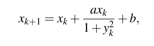
Inspired by Refs. [31-33], we construct a new class of two-dimensional rational maps in the following form:

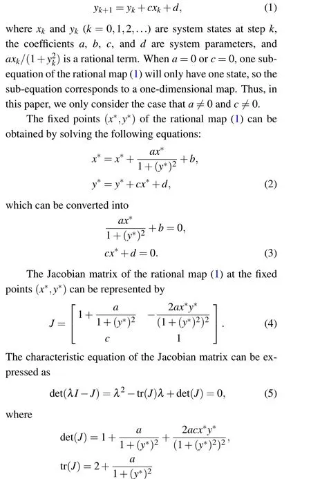
stand for the determinant of the Jacobian matrix and the trace of the Jacobian matrix,respectively. Eigenvalues ofJ,λ1,andλ2are termed as multipliers of the fixed point. Denote the numbers of multipliers of the fixed point(x*,y*)lying inside,on and outside the unit circle{λ ∈C:|λ|=1}byn-,n0,andn+, respectively. The fixed point is stable if the roots of the characteristic equationλ1andλ2satisfy that|λ1,2|＜1,where|·|refers to the modulus of a complex number.

Definition 1 (Definition 2.10 in Ref. [42]) A fixed point(x*,y*) is called hyperbolic ifn0=0, that is, if there is no eigenvalue of the Jacobian matrix evaluated at this fixed point on the unit circle. Otherwise, the fixed point is called nonhyperbolic,that is,there is at least one eigenvalue of the Jacobian matrix evaluated at the fixed point on the unit circle.

To distinguish the hidden and self-excited attractors of the rational map(1),the following definition is introduced.

Definition 2[43]An attractor is called a hidden attractor if its basin of attraction does not intersect with the small neighborhoods of equilibria(fixed points)of the system(map);otherwise,it is called a self-excited attractor.

Five cases can be divided from Eq.(2)as follows.

Ifa/=0,b=0,c/=0, there are two different cases, i.e.,d=0 andd/=0.

Case I:a/=0,b=0,c/=0,d=0(a line of fixed points).

Whena/=0,b=0,c/=0, andd=0, there is a line of fixed points(0,e),e ∈R. The Jacobian matrix of the rational map(1)at the fixed points(0,e)can be rewritten as

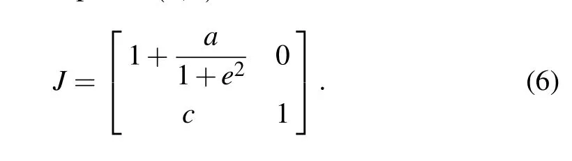
The multipliers of the fixed points, eigenvalues ofJ,λ1=1 andλ2=1+a/(1+e2). Thus,according to definition 1,these fixed points are all non-hyperbolic.Then these fixed points are critical stable.

Case II:a/=0,b=0,c/=0,d/=0(no fixed point A).

Whena/=0,b=0,c/=0, andd/=0, Eq. (2) has none solution. So there is no fixed point.

Ifa/=0,b/=0,andc/=0,thenx*=-d/c,-ad/[c(1+(y*)2)]+b=0,i.e.,(y*)2=(ad/bc)-1. So ifa/=0,c/=0,andb/=0,three cases can be obtained by considering the size relation between(ad/bc)and 1.

Case III:a/=0,b/=0,c/=0,(ad/bc)＜1(no fixed point B).

Whena/=0,b/=0,c/=0, and(ad/bc)＜1, Eq.(2)has none solution. So there is no fixed point.

Case IV:a/= 0,b/= 0,c/= 0, (ad/bc) = 1 (one fixed point).

Whena/=0,b/=0,c/=0, and(ad/bc)=1, Eq.(2)has two equal solutions,i.e.,x*=-d/c,y*=0. So there is only one fixed point. The Jacobian matrix of the rational map(1)at the fixed point(-d/c,0)can be expressed as

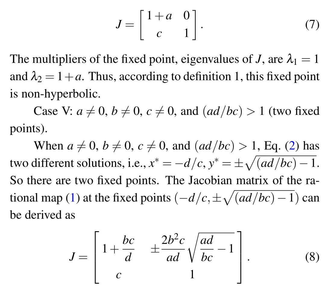
The multipliers of the fixed points can also be obtained by solving the characteristic equation of the Jacobian matrix(8),which will be analyzed in the following section.

3. Dynamical behaviors of the rational map

There are several ways to construct a bifurcation diagram,for example, by using random or fixed initial value, and forward or backward. In the random bifurcation diagram, many initial values are selected randomly in a range for each bifurcation parameter value. So the random bifurcation diagram can be used to exhibit all possible attractors. In the forward(backward)bifurcation diagram,one initial value is chosen first and the method of “follow the attractor” is used, that is, the last steady state is used for the initial state of next value of the increasing(decreasing)bifurcation parameter. In the bifurcation diagram calculated by using the fixed initial value,only a fixed initial value is chosen for all the values of the bifurcation parameter.

In this section, the dynamical behaviors of the rational map (1) will be investigated in five cases in accordance with different types of fixed points. In each case,the random bifurcation diagram[30]is drawn firstly to show the possible attractors of the rational map(1). If no multi-stability is observed,the forward(backward)bifurcation diagram will be presented to show the complex behaviors of the rational map(1). Moreover, the Lyapunov exponent spectrum (Les) and the Lyapunov (Kaplan-Yorke) dimension (Dky) of the attractors of the rational map(1)are computed by using the Wolf methods given in Refs.[14,44].

3.1. Case I:a line of fixed points

By random searching,chaotic attractors were found with several coefficients satisfying the condition thata/=0,b=0,c/=0, andd=0, i.e., there exist a line of fixed points. For example,whena=-3,b=0,c=0.1,andd=0,the rational map(1)can present chaotic attractors.

In order to show the complex dynamics of the rational map (1) with a line of fixed points, random bifurcation diagram and Lyapunov exponent spectrum diagram of the map were plotted in Fig. 1 by usingaas a branching parameter and fixing (b,c,d) as (0,0.1,0), where 500 initial values were randomly chosen within [-5,5] for each value of the parametera. The steady states after transience marked by black dots were shown in Fig.1(a),and the largest Lyapunov exponents (Le1) were indicated by black dots in Fig. 1(b).Since there were many fixed points, many Lyapunov exponents of the map for each parameter value were presented.To see the largest Lyapunov exponents clearly, the smallest Lyapunov exponents were omitted. Some samples of phase portraits of the rational map (1) with different values of the parameterawere presented in Fig. 2. As can be seen from Fig.1,when-4≤a ≤-1,the rational map(1)shows a line of fixed points (Fig. 2(a)). Asadecreases from-1 to-2, a period-2 solution(Fig.2(b))emerges. Whena=-2.667,the period-2 solution bifurcates to a period-8 solution(Fig.2(c)).Whena=-2.892, there is a reverse period-doubling bifurcation, and the period-8 solution bifurcates to a period-16 solution (Fig. 2(d)), and then becomes multiple-piece chaos(Fig. 2(e)) and two-piece chaos (Fig. 2(f)) after a reverse period-doubling cascade. Thereafter the map experiences a small window of periodic solutions (Fig. 2(g)). There is coexistence of stable fixed points,periodic solutions and chaotic solutions(Fig.2(h)). Finally, the two-piece chaotic attractors are merged into one-piece chaotic attractors(Fig.2(i)),which terminate to emerge ata=-3.38.

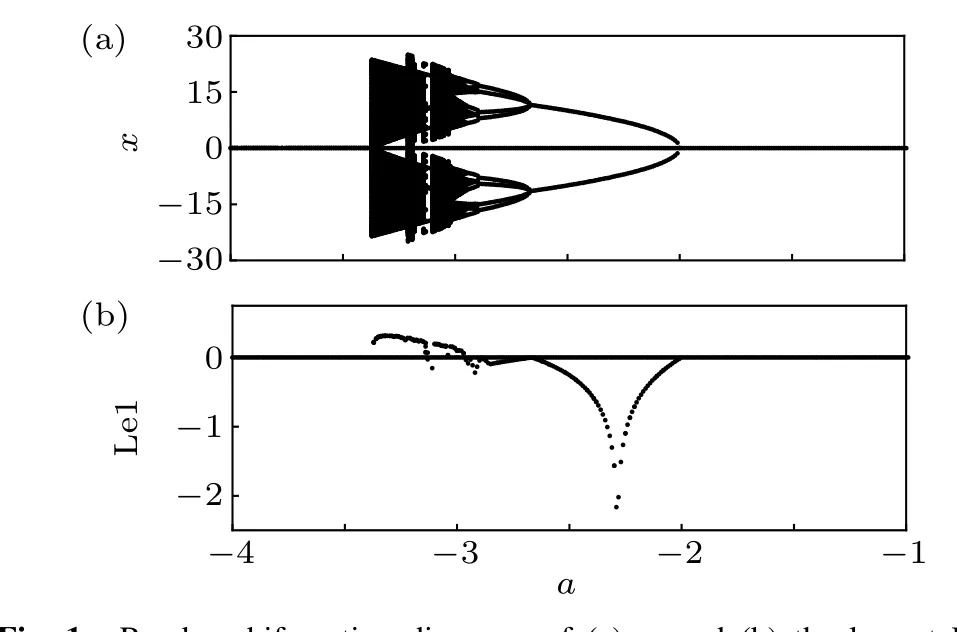
Fig. 1. Random bifurcation diagrams of (a) x, and (b) the largest Lyapunov exponent (Le1) of the rational map (1) calculated for a ∈[-4,-1]and (b,c,d)=(0,0.1,0). In Fig. 1(b), the horizontal line denotes the zero value of the largest Lyapunov exponent.

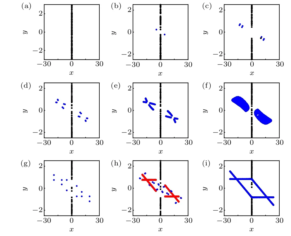
Fig. 2. Phase portraits of the solutions of the rational map (1) calculated at(b,c,d)=(0,0.1,0) and (a) a=-1.95 (stable fixed points), (b) a=-2.1(stable fixed points and period-2 solution),(c)a=-2.7(stable fixed points and period-8 solution), (d) a=-2.9 (stable fixed points and period-16 solution),(e)a=-2.98(stable fixed points and eight-piece chaotic solution),(f) a = -3.05 (a line of fixed points and two-piece chaotic solution), (g)a = -3.11 (stable fixed points and period-12 solution), (h) a = -3.135(stable fixed points, period-24 solution and four-piece chaotic solution), (i)a=-3.37(stable fixed points and one-piece chaotic solution),respectively.

To show the stability of a line of fixed points,we plotted the basin of attraction of the rational map(1)whena=-3.05,b=0,c=0.1,andd=0 as shown in Fig.3.The black and red dots represent the chaotic attractor and the stable fixed points,respectively. The basins of the chaotic attractor, the stable fixed points and unbounded solutions were painted cyan,yellow and white, respectively. From Fig. 3, although the line of fixed points are all non-hyperbolic, many fixed points are stable while there exist unstable fixed points. Since the knowledge about the line of fixed points is not very helpful for the localization of attractors,the attractors with a line of fixed points can also be considered as hidden attractors.

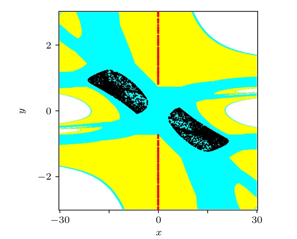
Fig.3. Basins of attraction of the rational map(1)when a=-3.05, b=0,c=0.1,d=0 in the region{(x,y)|x ∈[-30,30],y ∈[-3,3]}.The unbounded basin of attraction which is the set of initial points going into the region({(x,y)||x|+|y|＞100}) is shown in white. The chaotic attractor, the stable fixed points and unstable fixed points are denoted by black,red and blue dots,respectively. The basin of chaotic attractors and stable fixed points are shown in cyan and yellow,respectively.

3.2. Case II:no fixed point A

By random searching,chaotic attractors were found with several coefficients satisfying the condition thata/=0,b=0,c/=0,andd/=0,i.e.,there exists no fixed point. So the attractors are hidden. For example,whena=-3,b=0,c=1,andd=0.1,the rational map(1)has chaotic attractors.

To show the complex dynamics of the rational map (1)with no fixed point, forward bifurcation diagram and Lyapunov exponent spectrum diagrams of the map were plotted in Fig.4 by usingaas a varying parameter and fixing(b,c,d)as (0,1,0.1), where the initial value was assigned as (1,0),and the final state at the end of each iteration of the parameter was used as the initial state for the next iteration of computation. The steady states after transience denoted by black dots were presented in Fig.4(a),and the largest Lyapunov exponent (Le1), the smallest Lyapunov exponent (Le2) and the Lyapunov(Kaplan-Yorke)dimension(Dky)were indicated by red,blue and black lines in Fig.4(b),respectively.From Fig.4,the Lyapunov exponent spectrum diagram is in good agreement with the bifurcation diagram. Figure 5 presents some samples of phase portraits of the solutions for the rational map(1). It can be seen from Fig.4 that,whena=-2.361,the rational map(1)shows a hidden period-2 solution(Fig.5(a)).Asadecreases to-2.521, the rational map(1)experiences a reverse period-doubling bifurcation, and the hidden period-2 solution bifurcates to a hidden period-4 solution (Fig. 5(b)).Whena=-2.741, another reverse period-doubling bifurcation is encountered,and this hidden period-4 solution converts into a hidden period-8 solution (Fig. 5(c)). Ata=-2.798,this hidden period-8 solution transforms into a hidden period-16 solution(Fig.5(d)),and then becomes multiple-piece chaos after a reverse period-doubling cascade. After that, a small window of hidden period-6 solutions (Fig. 5(e)) and hidden period-12 solutions are recorded, and the rational map (1)goes into chaotic states again ata=-2.965 through a reverse period-doubling cascade. Finally,whena=-3.144,the hidden two-piece chaotic attractors are jointed together into hidden one-piece chaotic attractors(Fig.5(f)),which disappear ata=-3.148.

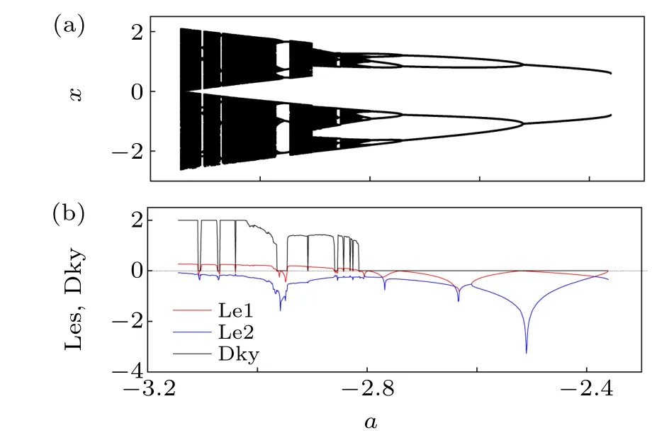
Fig. 4. Forward bifurcation diagram of (a) x, and (b) Lyapunov exponent spectrum(Les)and Lyapunov(Kaplan-Yorke)dimension(Dky)of the rational map(1)calculated for a ∈[-3.2,-2.3]and(b,c,d)=(0,1,0.1)using the initial value(1,0). The largest Lyapunov exponent(Le1), the smallest Lyapunov exponent (Le2) and the Lyapunov (Kaplan-Yorke) dimension (Dky)are indicated by red,blue and black lines,respectively.The dashed horizontal line denotes that the zero value of the Lyapunov exponent and the Lyapunov(Kaplan-Yorke)dimension.

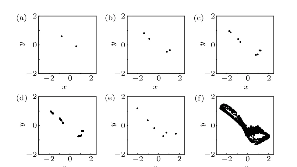
Fig. 5. Phase portraits of the solutions of the rational map (1) calculated at (b,c,d)=(0,1,0.1) and (a) a=-2.361 (hidden period-2 solution), (b)a=-2.600(hidden period-4 solution),(c)a=-2.780(hidden period-8 solution),(d)a=-2.817(hidden period-16 solution),(e)a=-2.946(hidden period-6 solution), (f) a=-3.144 (one-piece hidden chaotic solution), respectively.

3.3. Case III:no fixed point B

Whena=-3,b=1,c=-0.1, andd=-0.1, the condition thatb/=0 and(ad/bc)＜1 is fulfilled, i.e., there is no fixed point. So the attractors are hidden. Ifb=1,c=-0.1,d=-0.1, anda ＜1, then (ad/bc)＜1, so there is no fixed point and the attractors are hidden.

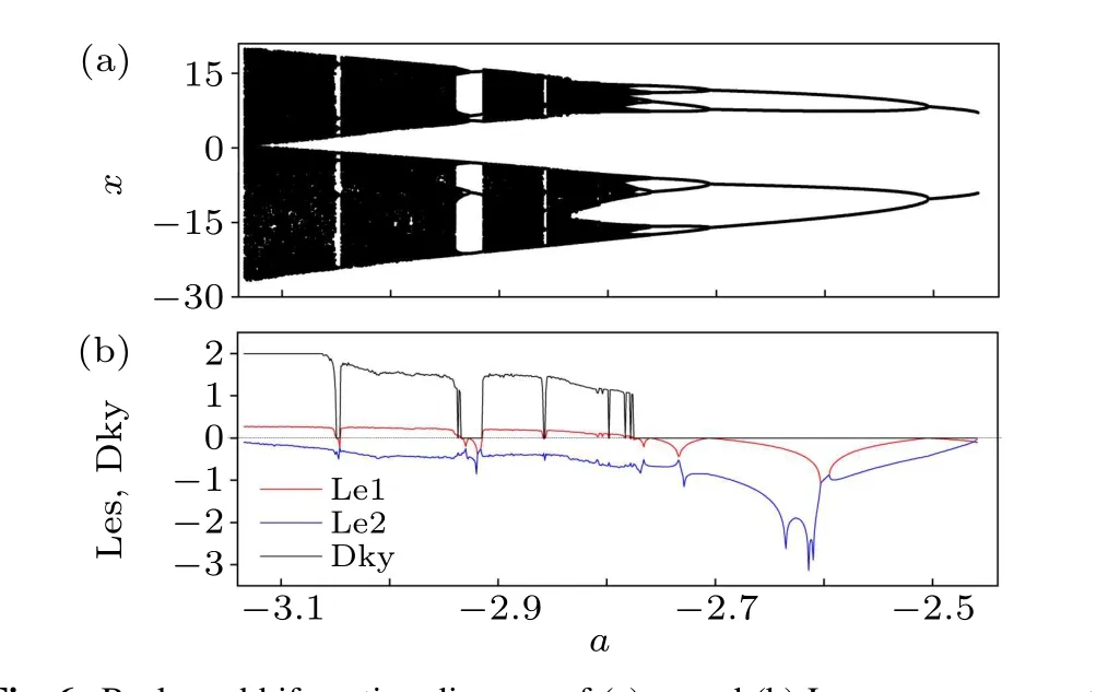
Fig. 6. Backward bifurcation diagram of (a) x, and (b) Lyapunov exponent spectrum(Les)and Lyapunov(Kaplan-Yorke)dimension(Dky)of the rational map(1)calculated for a ∈[-3.14,-2.44]and(b,c,d)=(1,-0.1,-0.1)using the initial value (7,0). The largest Lyapunov exponent (Le1), the smallest Lyapunov exponent (Le2) and Lyapunov (Kaplan-Yorke) dimension(Dky)are denoted by red,blue and black lines,respectively. The dashed horizontal line denotes the zero value of the Lyapunov exponent and the Lyapunov(Kaplan-Yorke)dimension.

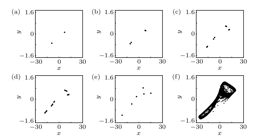
Fig. 7. Phase portraits of the solutions of the rational map (1) calculated at(b,c,d)=(1,-0.1,-0.1)and(a)a=-2.459(hidden period-2 solution),(b)a=-2.508(hidden period-4 solution),(c)a=-2.718(hidden period-8 solution),(d)a=-2.776(hidden period-16 solution),(e)a=-2.926(hidden period-6 solution), (f) a=-3.133 (one-piece hidden chaotic solution),respectively.

In order to show the complex dynamics of the rational map (1) with no fixed point, backward bifurcation diagram and Lyapunov exponent spectrum diagram of the map were depicted in Fig. 6 by usingaas a bifurcation parameter and fixing(b,c,d)as(1,-0.1,-0.1). The initial value was set as(7,0)and the final state at the end of each iteration of the parameter was used as the initial state for the next iteration of computation. The steady states after transience were shown in Fig.6(a),and the largest Lyapunov exponent(Le1),the smallest Lyapunov exponent (Le2) and the Lyapunov (Kaplan-Yorke)dimension(Dky)were denoted by red,blue and black lines in Fig. 6(b), respectively. From Fig. 6, the Lyapunov exponent diagram agrees well with the bifurcation diagram.Figure 6 presents some samples of phase portraits of the solutions for the rational map(1).It is apparent from Fig.6 that the bifurcation procedure of case III is very similar to that of Case II. Whena=-2.459, a hidden period-2 solution (Fig. 7(a))exists. Asadecreases to-2.504, there is a reverse perioddoubling bifurcation, leading the hidden period-2 solution to a hidden period-4 solution (Fig. 7(b)). Whena=-2.706,the occurrence of another reverse period-doubling bifurcation leads the hidden period-4 solution to a hidden period-8 solution (Fig. 7(c)). Ata=-2.760, this hidden period-8 solution becomes a hidden period-16 solution (Fig. 7(d)),and then changes into hidden multiple-piece chaos after a reverse period-doubling cascade. Hereafter, the map exhibits a small window of hidden period-6 solutions (Fig. 7(e)) and hidden period-12 solutions,and bifurcates into chaos again ata=-2.937 via a reverse period-doubling cascade.Finally,the hidden two-piece chaotic attractors are combined into hidden one-piece chaotic attractors(Fig.7(f)),which cease to exist ata=-3.158.

3.4. Case IV:a single fixed point

By random searching, several coefficients satisfying the condition thatb/=0,(ad/bc)=1 and yielding chaotic attractors of the rational map(1)were found. In this case,the rational map(1)has a single non-hyperbolic fixed point.Ifa=-3,b=1,c=0.6, andd=-0.2, the non-hyperbolic fixed point is (1/3,0) and the map shows a two-piece chaotic attractor with the initial value chosen as (0,0). Figures 8(a) and 8(b)show the statesxandyof the chaotic attractor of the rational map (1) as a function of the stepk, respectively. Figure 8(c)presents the phase portrait of the chaotic attractor of the rational map(1). Based on our numerical computation,Lyapunov exponent spectrum (Les) of the chaotic attractor are 0.2182,-0.1304,and its Lyapunov(Kaplan-Yorke)dimension(Dky)is 2,which proves the chaotic property of the rational map(1).

The basin of attraction of the rational map (1) was depicted in Fig. 9. The cyan and white regions correspond to the basin of the chaotic attractor and the unbounded solution,respectively. The black dots and the blue dot represent the chaotic attractor and the non-hyperbolic fixed point, respectively. From Fig.9,the non-hyperbolic fixed point lies inside the chaotic attractor’s basin,so the initial values chosen from any small punctured neighborhood of the fixed point will tend to the chaotic attractor. However, the basin of the chaotic attractor exhibits to be striped.

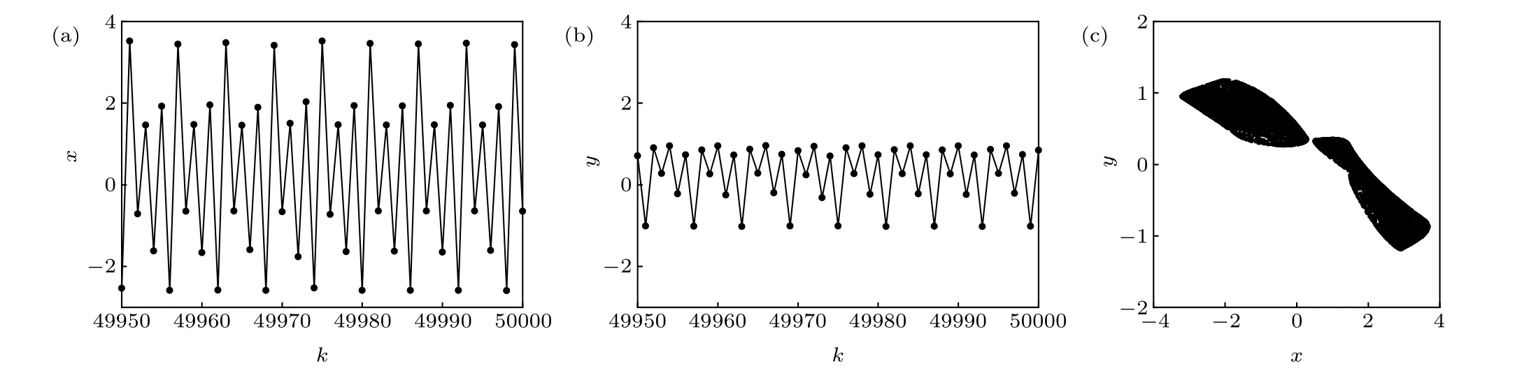
Fig. 8. Time histories of (a) x, (b) y, and (c) phase portrait of the chaotic attractor of the rational map (1) calculated by using the parameter (a,b,c,d)=(-3,1,0.6,-0.2)and the initial value(0,0).

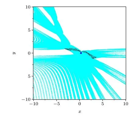
Fig. 9. Basins of attraction of the rational map (1) when a=-3, b=1,c = 0.6, and d = -0.2 in the region {(x,y)|x ∈[-10,10],y ∈[-10,10]}.The chaotic attractor and the non-hyperbolic fixed point are denoted by black dots and a blue dot, respectively. The basin of the chaotic attractor and the unbounded solution are shown in cyan and white,respectively.

3.5. Case V:two fixed points

Ifb/=0 and (ad/bc)＞1, the rational map (1) has two fixed points. By numerical exploration,the stabilities of these fixed points can be classified into two cases, i.e., one stable and one unstable fixed points,and two unstable fixed points.In the following,we will discuss these cases in detail.

3.5.1. Case VA: one stable and one unstable fixed points

Ifa=-3,b=1,c=0.1,andd=-0.1,thenb/=0 and(ad/bc)＞1,i.e.,there are two fixed points. Ifb=1,c=0.1,d=-0.1,anda ＜-1,then(ad/bc)＞1,there are two fixed points.

In order to show the complex dynamics of the rational map (1) with two fixed points, random bifurcation diagram and Lyapunov exponent spectrum diagram of the map were presented in Fig. 10 by varyingain the range [-4,-1] and fixing (b,c,d) as (1,0.1,-0.1), where 500 initial states were randomly selected in the interval[-5,5]for each value of the parametera. The steady states after transience marked by black dots were shown in Fig. 10(a). The largest Lyapunov exponent (Le1) and the smallest Lyapunov exponent (Le2)were indicated by red and blue dots in Fig.10(b),respectively.According to Fig. 10, there is a good agreement between the Lyapunov exponent spectrum diagram and the bifurcation diagram. When-4＜a ＜-1,there are one unstable fixed point(UFP) and one stable fixed point (SFP), represented by blue dashed lines and red lines, lying in down and up branches,respectively. Asaincreases to-1, the stable and unstable branches intersect and the stable fixed point becomes unstable via a saddle-node bifurcation. Figure 11 presents some samples of phase portraits of the solutions for the rational map (1). For-2.361＜a ＜-1, there only exists one stable fixed point(Fig.11(a)). Whena=-2.361,the map(1)shows a coexisting period-2 solution (Fig. 11(b)). Asadecreases to-2.521, a reverse period-doubling bifurcation occurs, and the coexisting period-2 solution loses stability,leaving a coexisting period-4 solution (Fig. 11(c)). Whena=-2.741, another reverse period-doubling bifurcation arises, and this coexisting period-4 solution bifurcates to a coexisting period-8 solution(Fig.11(d)),and then becomes a coexisting multiplepiece chaotic attractor (Fig. 11(e)) through a reverse perioddoubling cascade. Some small range in which there are more than three coexisting attractors are observed, e.g., the coexistence of fixed point, period-6 solution and chaotic attractor(Fig.11(f)). After that,a cascade of period-doubling bifurcations is observed and the state of the map(1)goes to the coexisting period-8 solution(Fig.11(g)),which evolves into chaos again as a result of a reverse period-doubling cascade. Finally,whena=-3.14,the two-piece chaotic attractors(Fig.11(h))are formed into one-piece chaotic attractors(Fig.11(i)).When-4＜a ＜-3.38,there only exists one stable fixed point.

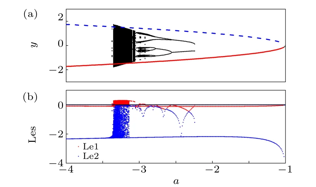
Fig. 10. Random bifurcation diagram of (a) x, and (b) Lyapunov exponent spectrum(Les)of the rational map(1)calculated for a ∈[-4,-1]and(b,c,d)=(1,0.1,-0.1). The stable fixed points(SFP),unstable fixed points(UFP) and attractors expect for the stable fixed points are denoted by red lines,dashed lines and black dots,respectively. The largest Lyapunov exponent (Le1) and the smallest Lyapunov exponent (Le2) are indicated by red and blue dots,respectively. In Fig.10(b),the horizontal line denotes the zero value of the Lyapunov exponent.

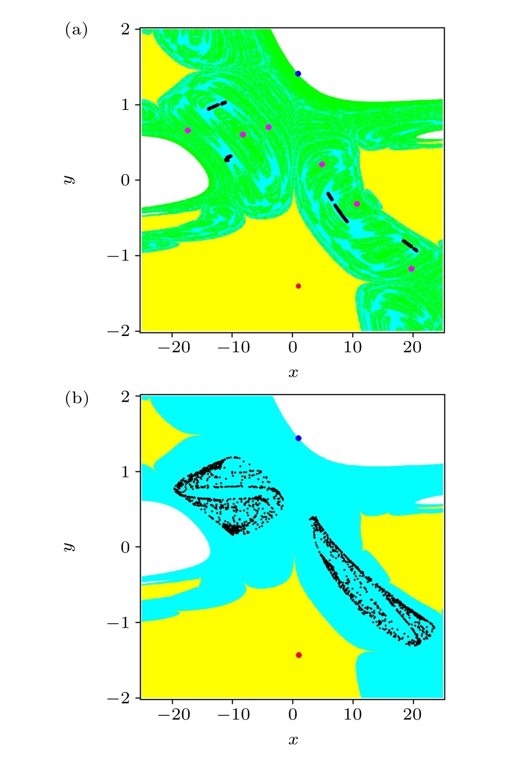
Fig.12. Basins of attraction of the rational map(1)when(a)a=-2.98,(b)a=-3.06 and b=1,c=0.1,d=-0.1 in the region{(x,y)|x ∈[-25,25],y ∈[-2,2]}. The chaotic attractor, the period-6 attractor, the stable fixed point and the unstable fixed point are represented by black,magenta,red and blue dots,respectively. The basins of the chaotic attractors,the period-6 attractor,the stable fixed point and the unbounded solution are shown in cyan,green,yellow and white,respectively.

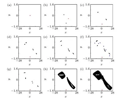
Fig.11. Phase portraits of the solutions of the rational map(1)calculated at(b,c,d)=(1,0.1,-0.1)and(a)a=-1(a fixed point),(b)a=-2.24(fixed point and period-2 solution), (c) a=-2.56 (fixed point and period-4 solution),(d)a=-2.79(fixed point and period-8 solution),(e)a=-2.94(fixed point and chaotic solution),(f)a=-2.98(one fixed point,period-6 solution and chaotic solution),(g)a=-3.04(fixed point and period-8 solution),(h)a=-3.06(fixed point and two-piece chaotic solution),(i)a=-3.14(fixed point and one-piece chaotic solution),respectively.

To show the hidden and self-excited attractors of the rational map(1),we computed the basin of attraction of the map whena=-2.98 anda=-3.06,b=1,c=0.1,d=-0.1,as demonstrated in Fig.12,respectively. The chaotic attractor,the period-6 attractor, the stable fixed point and the unstable fixed point were represented by black, magenta, red and blue dots, respectively. The basins of the chaotic attractors,the period-6 attractor, the stable fixed points and the unbounded solutions were colored in cyan, green, yellow and white, respectively. From Fig.12(a), the period-6 attractor is self-excited since one unstable fixed point stays in the basin of the period-6 attractor. However,the chaotic attractor is hidden since the basin of the chaotic attractor is not connected with any small neighborhoods of the fixed points. It can be concluded from Fig.12(b)that,the chaotic attractor is self-excited since one unstable fixed point lies in the basin of the chaotic attractor, i.e., the basin of the chaotic attractor is connected with the small neighborhoods of the unstable fixed point.

3.5.2. Case VB: two unstable fixed points

Ifa=-1,b=-1,c=1,andd=2,then we haveb/=0 and(ad/bc)＞1,i.e.,there exist two fixed points. Ifa=-1,c=1,d=2 and-2＜b ＜0, then (ad/bc)＞1. Thus the rational map(1)admits two fixed points. In the following,we chosea=-1,c=1,d=2, and selectedbas a branching parameter. Figure 13 presents the fixed points of the rational map (1) calculated forb ∈[-2.1,-0.01] and (a,c,d)=(-1,1,2). The stable and unstable fixed points were indicated by red and blue lines,respectively.For-2.1＜b ＜-2,there is an unstable fixed point. Then the rational map(1)experiences a saddle-node bifurcation atb=-2, which yields one stable fixed point and one unstable fixed point. When the parameterbincreases to-1.867, the stable fixed point loses stability and becomes unstable through a saddle-node bifurcation.When the parameterbincreases further, this unstable fixed point gains stability and becomes stable atb=-0.133 via a saddle-node bifurcation. Thus there are two unstable fixed points forb ∈[-1.866,-0.132].

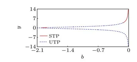
Fig. 13. The fixed points of the rational map (1) calculated for b ∈[-2.1,-0.001]and(a,c,d)=(-1,1,2).The stable and unstable fixed points are indicated by red and blue lines,respectively.

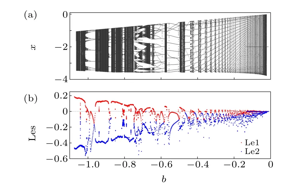
Fig. 14. Random bifurcation diagram of (a) x, and (b) Lyapunov exponent spectrum(Les)of the rational map(1)calculated for b ∈[-1.1,-0.001]and(a,c,d)=(-1,1,2) using the initial value randomly chosen in the interval[-5,5]. The largest Lyapunov exponent (Le1) and the smallest Lyapunov exponent(Le2)are indicated by red and blue dots,respectively. The dashed horizontal line denotes the zero value of the Lyapunov exponent.

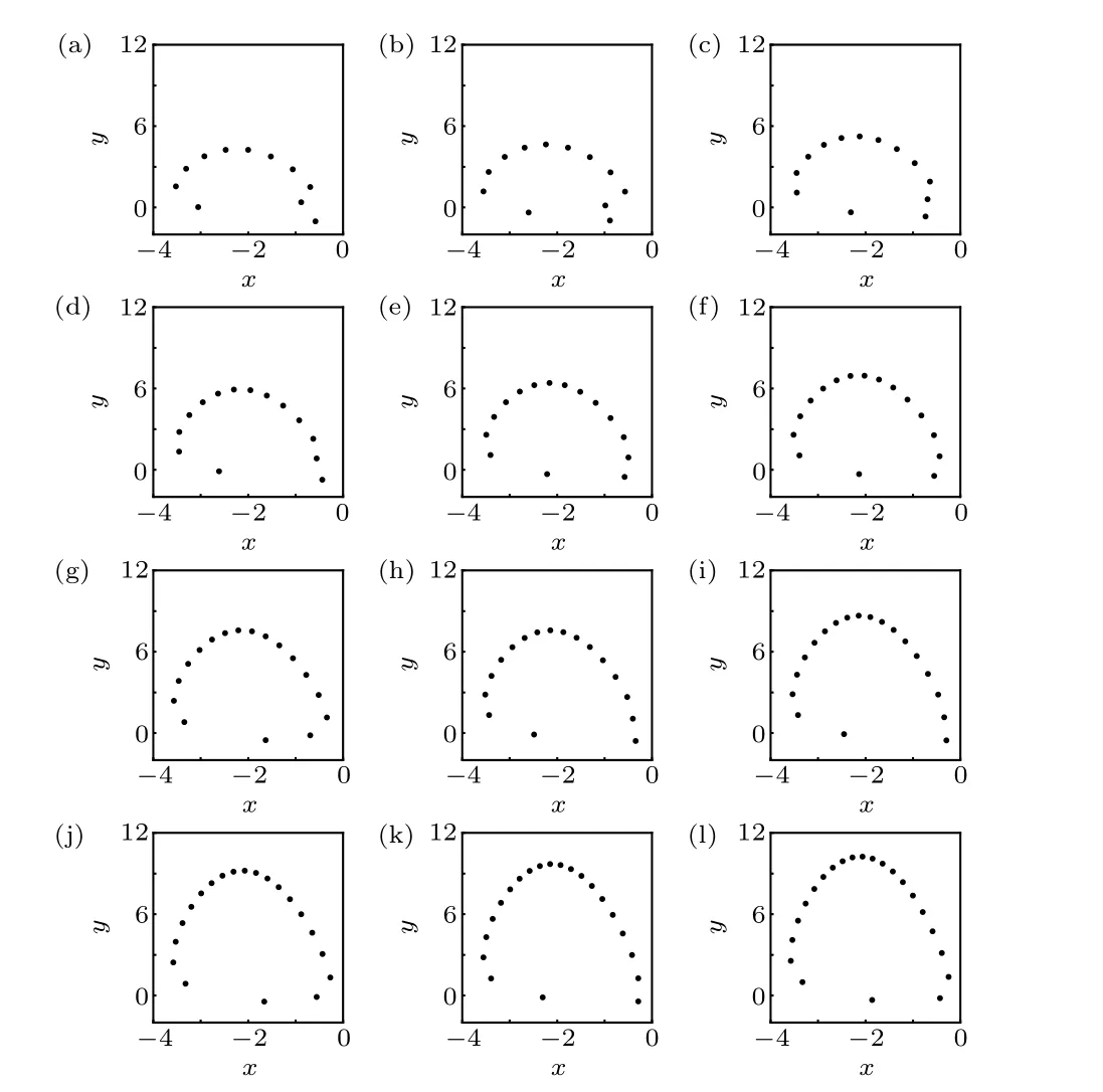
Fig.15. Phase portraits of the solutions of the rational map(1)calculated at(a,c,d)=(-1,1,2)and(a)b=-0.58(period-11 solution), (b)b=-0.55(period-12 solution), (c) b = -0.46 (period-13 solution), (d) b = -0.40(period-14 solution), (e) b = -0.37 (period-15 solution), (f) b = -0.34(period-16 solution), (g) b = -0.32 (period-17 solution), (h) b = -0.31(period-18 solution), (i) b = -0.27 (period-19 solution), (j) b = -0.26(period-20 solution), (k) b = -0.24 (period-21 solution), (l) b = -0.23(period-22 solution),respectively.

For showing the complex dynamics of the rational map (1) with two fixed points, random bifurcation diagram and Lyapunov exponent spectrum diagram of the map were illustrated in Fig. 14 by takingbas a control parameter and fixing (a,c,d) as (-1,1,2), where 500 initial states were randomly selected in the interval [-5,5] for each value of the parameterb. The steady states after transience were depicted in Fig. 14(a). The largest Lyapunov exponent (Le1)and the smallest Lyapunov exponent (Le2) were indicated by red and blue dots in Fig.14(b),respectively. From Fig.14,the Lyapunov exponent diagram coincides with the bifurcation diagram. Figure 15 presents some samples of phase portraits of the solutions for the rational map (1). It is apparent from Fig. 14 that, there exist many chaotic regimes and periodic windows. For-0.58≤b ＜0, the period of the periodic solutions increases by one from eleven, as displayed in Figs. 15(a)-15(l), which can be considered as periodadding bifurcation. And the length of the chaotic regimes becomes shorter as the parameteraincreases. For-1.2＜b ＜-0.58, several period-doubling bifurcations and inverse period-doubling bifurcations are observed.Finally,the chaotic attractors disappear atb=-1.075. Although there exist two unstable fixed points, the rational map (1) may also exhibit hidden attractors.

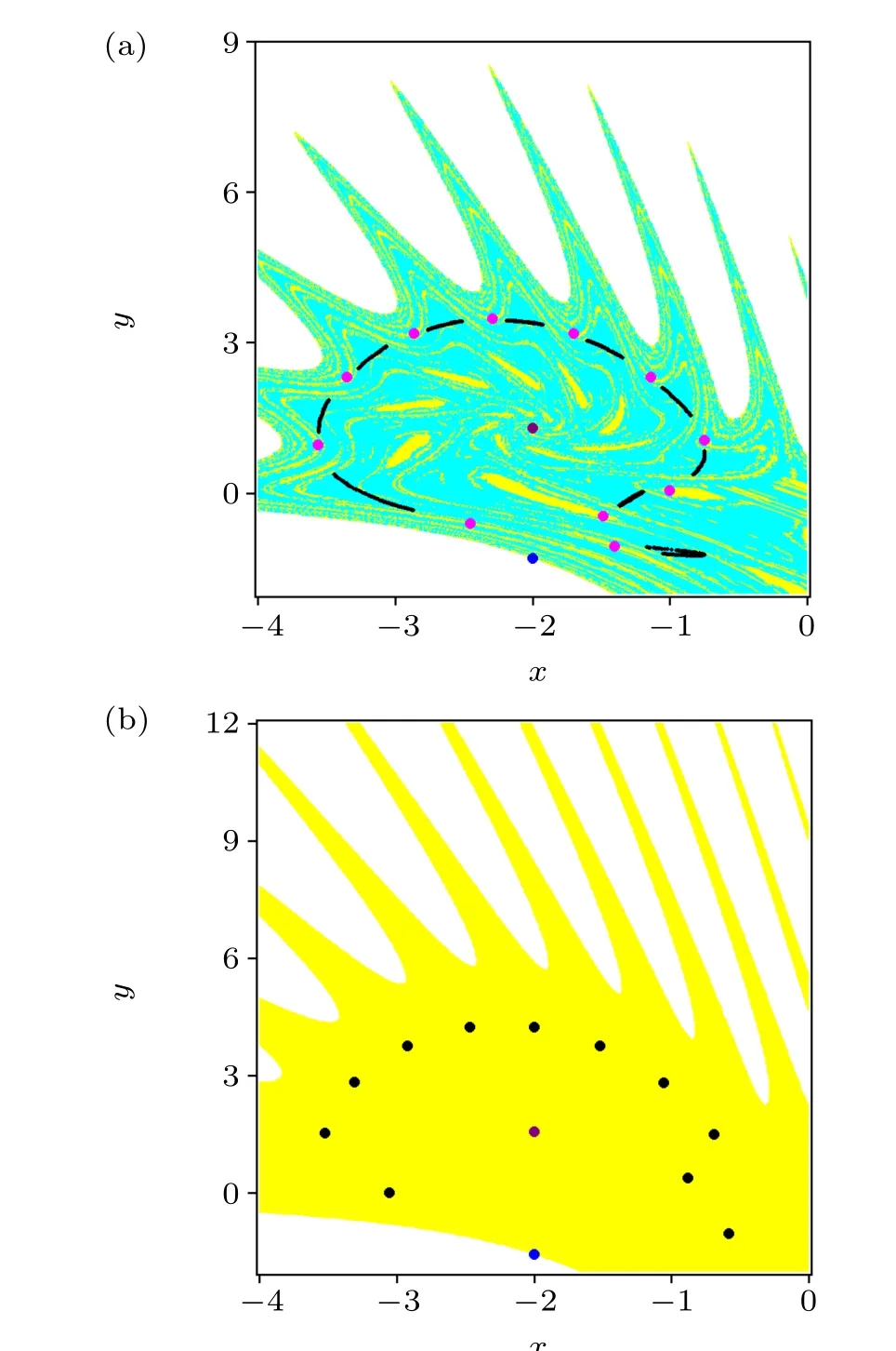
Fig. 16. Basins of attraction of the rational map (1) when (a) b=-0.745,(b)b=-0.58 and a=-1,c=1,d=2,respectively. The chaotic attractors,the period-11 attractor,the stable fixed point and the unstable fixed point are denoted by black, magenta, red and blue dots, respectively. The basins of the chaotic attractors, the period-11 attractor, the stable fixed point and the unbounded solution are shown in cyan,green,yellow and white,respectively.

To distinguish the hidden and self-excited attractors of the rational map (1), we drew the basin of attraction of the map(1)forb=-0.745 andb=-0.58,a=-1,c=1,d=2,as demonstrated in Fig.16. The chaotic attractor, the period-6 attractor, the stable fixed point and the unstable fixed point were represented by black, magenta, red and blue dots, respectively. The basins of the chaotic attractors, the period-11 attractor, the stable fixed points and the unbounded solutions were colored in cyan, green, yellow and white, respectively.From Fig.16(a), the basins of the period-11 attractor and the chaotic attractor are fractal,so the basins of the chaotic attractor and period-11 attractor are connected with the small neighborhoods of the fixed points.Hence the period-11 attractor and the chaotic attractor are all self-excited. It can be found from Fig.16(b)that,the period-11 attractor is self-excited since one unstable fixed point lies in the basin of the period-11 attractor,i.e.,the basins of the period-11 attractor is connected with the small neighborhoods of the unstable fixed point. We also verified the class of attractors according to the definition of hidden and self-excited attractors by exploiting the numerical tools as follows. Firstly, we obtained two fixed points. Then we randomly chose initial points in a very small neighborhood(＜0.001) of these fixed points. Finally, some points could tend to these self-excited attractors.

4. Conclusions

A new class of two-dimensional rational maps with different types of fixed points was introduced and studied in this paper. The existence and stabilities of fixed points of the rational map were discussed. Several numerical analysis tools were employed to demonstrate the rich and complex dynamics of the rational map. Both self-excited and hidden attractors were shown and explored in the rational map. In addition,multi-stability, especially the hidden multi-stability, was further investigated. The proposed rational map can be applied to secure network communications, such as data and image encryption.[32]Future works will focus on the investigation of high-dimensional rational maps with self-excited and hidden attractors.

Acknowledgments

Project supported by the National Natural Science Foundation of China (Grant Nos. 11672257, 11772306,11972173, and 12172340) and the 5th 333 High-level Personnel Training Project of Jiangsu Province of China (Grant No.BRA2018324).