
Three-dimensional coupled-mode model and characteristics of low-frequency sound propagation in ocean waveguide with seamount topography
2022-08-31 09:55:12YaXiaoMo莫亞梟ChaoJinZhang張朝金LiChengLu鹿力成andShengMingGuo郭圣明
Chinese Physics B 2022年8期
Ya-Xiao Mo(莫亞梟) Chao-Jin Zhang(張朝金) Li-Cheng Lu(鹿力成) and Sheng-Ming Guo(郭圣明)
1Key Laboratory of Underwater Acoustic Environment,Institute of Acoustics,Chinese Academy of Sciences,Beijing 100190,China
2China State Shipbuilding Corporation Systems Engineering Research Institute,Beijing 100094,China
Keywords: coupled-mode model,three-dimensional sound propagation,seamount topography,horizontal interference structure
1. Introduction
The presence of a favorable sound channel permits the ocean waveguide to effectively transmit a low-frequency sound field over a very long distance. For this reason, the International Monitoring System, with only six hydrophone stations, can effectively monitor the global ocean underwater nuclear emergency.[1]However, as a critical component of the ocean waveguide boundary, the submarine topography significantly influences the low-frequency sound transmission. According to the Wake Island hydrophone station,the Sarigan volcano eruption on May 29,2010,was effectively recorded and analyzed. The result showed that the predicted blockage from 2D propagation was over 40 dB greater than the observed blockage, which is caused by ignoring the lowfrequency acoustic diffraction effect in the prediction.[2]The horizontal refraction phenomenon in the South China Sea experiment was explained by using Bellhop3D, and the acoustic field structure in the horizontal refraction area was demonstrated to be considerably different from the result calculated by theN×2Dmodel.[3]
In the seamount environment,where horizontal refraction and diffraction become substantial,the conventional underwater acoustic field model[4]is also mostly limited, especially in the low-frequency range. Consequently, various 3D models, both analytic and numerical, have been researched. For instance, Y. T. Linet al.[5,6]developed a 3D parabolic equation model using a reasonable 3D root operator approximation. F.Sturm[7]confirmed the necessity of cross terms in the root operator approximation and showed that a leading-order cross-term correction could be sufficient to remove phase errors in 3D solutions. By introducing a perfectly matched layer method, C. X. Xuet al.[8]eliminated the truncated boundary in the horizontal direction in 3D Cartesian coordinates. The PE described above can effectively compute the sound field of the ocean waveguide, but it lacks clear physical meaning,and can not use directly those methods like mode analysis,[4]which are often supplemented to explain the propagation phenomena.
The couple-mode method has attracted considerable attention to analyze the low-frequency acoustic propagation phenomena. It explains the influence of variations in the volume parameters and topography on sound energy transmission by coupling normal modes.[9–12]Due to the continuous vertical displacement is used for the nonhorizontal interface with distinct sound impedance, the bathymetric contributions to ocean acoustic mode coupling matric elements are poorly in the traditional mode coupling theory. In order to solve this problem, O. A. Godin[13,14]developed a new derivation based on the reciprocity principle rather than the wave equation. Meanwhile,the acoustic reciprocity and the energy conservation are illustrated theoretically,and the results show that the antisymmetric coupling coefficients are necessary. In addition to a direct theoretical derivation to obtain the expression of the coupling coefficient to explain these influences,the deep network method[15]has also been introduced to build a random mode coupling matrix.However,for general problems,the numerical implementation for 3D coupled-mode solution is not as simple as for the 3D PE method. We often ignore the mode coupling or only use this method on a special topography. For example,the 3D coupled-mode parabolic equation method has a high computational efficiency at the expense of ignoring the coupling of azimuth angles.[16]A 3D coupled-mode model(FT-CM model) can be obtained by the Fourier transform to explain the topography effect,[17]but it is only applicable in the translationally invariant waveguide as wedge topography.Although the coupled model that does not ignore azimuth coupling in the seamount waveguide has been established,[18,19]it is still limited to symmetric situations. Therefore, a rigorous derivation of the 3D coupled-mode model is produced,and all mode couplings are contained in numerical implementation to analyze the 3D effect caused by the seamount and determine the low-frequency acoustic field. This paper is organized as follows. In Section 2, the coupled-mode model is derived.Then in Section 3, the model’s accuracy and the coupling is verified with the range-independent,the wedge and the conical seamount waveguides. The 3D effects such as horizontal refraction and diffraction caused by the seamount are discussed in Section 4. Conclusions are provided in Section 5.
2. The 3D coupled-mode model
2.1. Coupled differential eqnarray
In a 3D ocean waveguide with seamount topography(shown in Fig.1),the acoustic pressure fieldp(r,θ,z)and the particle displacement vector fieldu(r,θ,z) are excited by a point source at (0,0,zs). In cylindrical coordinates, the time factor exp(?iωt)is removed,and these physical fields satisfy
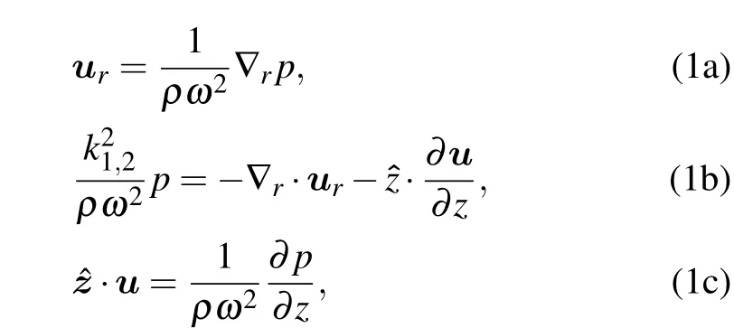
whereur=ur?r+uθ?θis the horizontal particle displacement vector. ?r, ?θ, and ?zrepresent the unit vectors in the direction ofr,θ, andz, respectively. Subscripts 1 and 2 of wavenumberk1,2=ω/c1,2indicate the water and bottom in the ocean waveguide, respectively. ?ris the Laplace operator in the(r,θ) plane, which acts on the scalar and vector and can be respectively expressed as
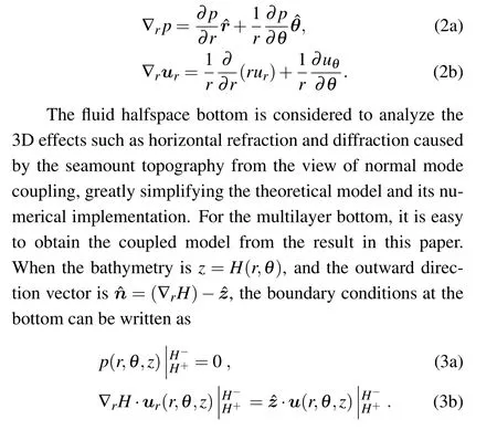
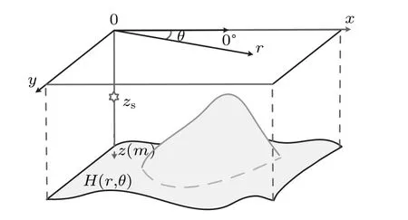
Fig. 1. Schematic diagram of 3D ocean waveguide with seamount topography.
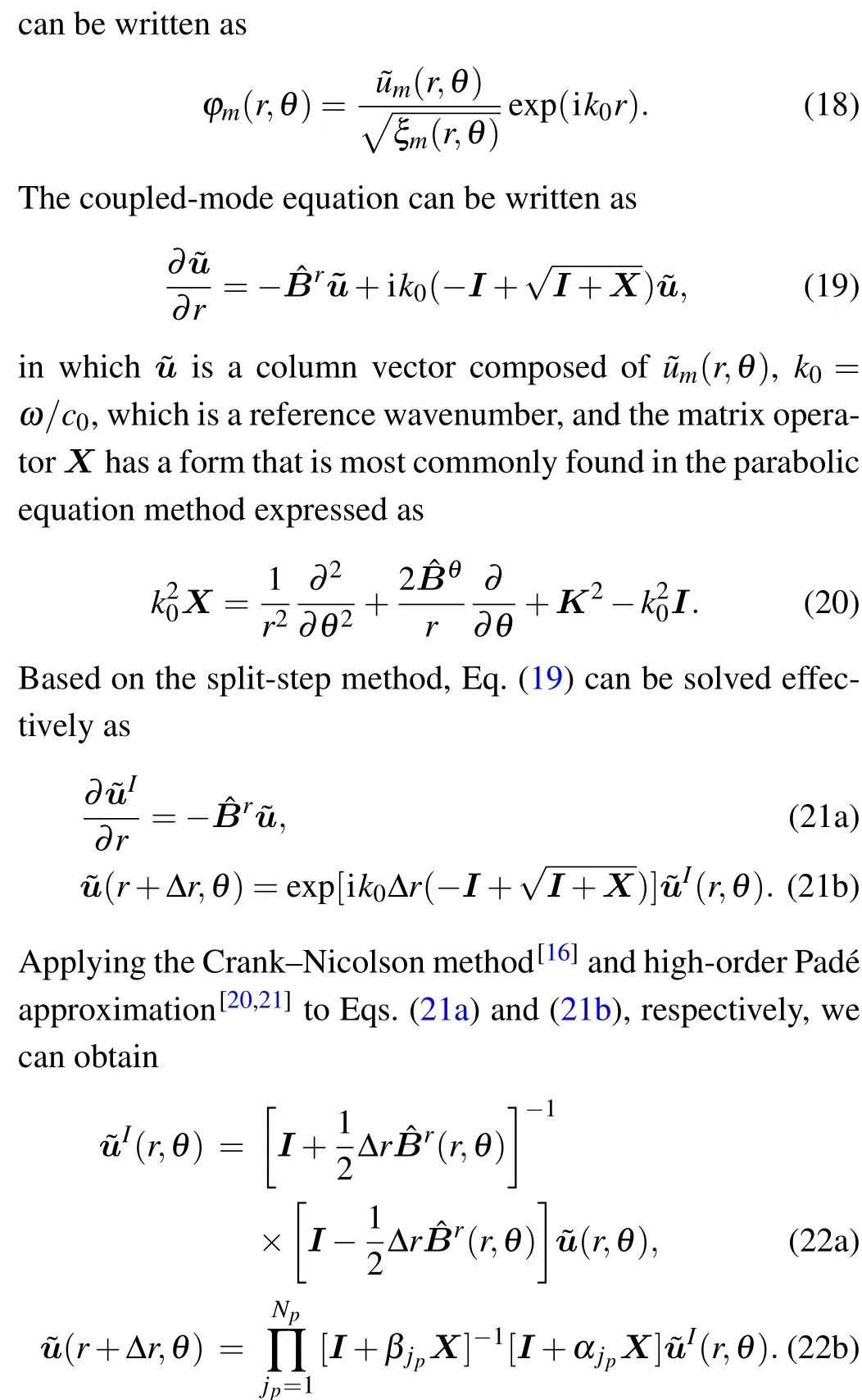
According to the normal mode theory,we can use the local vertical eigenfunctionφn(z;r,θ)as a basis function of the series expansion. The order of the series is infinite in theory.However,the leaky modes contribute much less as the ordernincreases. As a result,the physical field can be represented by the finite normal mode

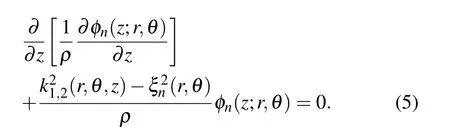
where?n(r,θ) and ??n(r,θ) are then-order coefficient of acoustic pressure and horizontal particle displacement vector in the normal mode expansion, respectively. They represent the mode amplitude and phase. The local eigenfunctionφn(z;r,θ) satisfies the local differential equation corresponding to the local eigenvalueξn(r,θ)
The bottom boundary conditions and the orthonormality satisfied by the eigenfunctionφn(z;r,θ)can be written as


Equations(7)and(11)have a first-order differential equation form and are called the fundamental coupled differential equation in the coupled model. ?BmnandBmnare the coupling coefficients in this form of the equation, and they are called the fundamental coupling coefficients, which can be easily verified to satisfy ?Bmn+Bnm= 0. According to the relation proposed by O. A. Godinet al.,[13,14]we can conclude that the coupled model represented by the fundamental differential equations satisfies the reciprocity and energy conservation in theory.
However,the fundamental coupled differential equations are difficult to solve numerically. For this reason, these coupled equations should be further simplified. When the vector operator ??ris applied to both sides of Eq.(7),subtracting Eq.(11),we can obtain a high-order coupled differential equation for them-order mode expansion coefficient?m(r,θ) and can be written as

In the coupling coefficient vector ?Bmn, the last term was obtained by using the nonhorizontal bottom boundary condition in Eq. (3b). It indicates that the effect of the bottom topography can be accurately considered. As a result,the coupling coefficient satisfies the antisymmetric relation ?Bmn=??Bnm.This antisymmetric can reduce computational efforts. Meanwhile,it can also guarantee that this model satisfies the energy conserved and is reciprocal in theory. Based on the definition of the vector operator ??r,the coupling coefficient vector ?Bmncan be expressed as the scalar form of the coupling coefficient in the(r,θ)plane

The influence of variations can be explained in the volume parameters and topography on sound energy transmission from the normal mode coupling by using the coupling coefficientsBrmn,Bθmn, andAmn. Moreover, the influence of the environment nonhorizontal variation can be effectively separated by the coupling coefficients along the orthogonality direction.This is beneficial for analyzing the sound propagation characteristics along a different horizontal direction. Besides them-order mode self-variation caused by the environment nonhorizontal variation,Eq.(13)can influence the coupling transmission from the other mode. When the coupling is neglected,the differential equation corresponds to the adiabatic approximation in the acoustic field theory.
2.2. The numerical implementation for the 3D coupledmode model
For the 3D coupled-mode model described by Eq.(13),a matrix differential equation can be obtained and written as

The derivation indicates that this model has the advantages of the coupled mode and parabolic equation theory. The couplings are fully included and effectively separated,the numerical implementation is also kept feasible. Moreover,by using higher-order Pad′e approximations,[20,21]the wide propagation horizontal angles can be obtained in the 3D result.
We consider the discrete form to solve Eq. (22) numerically, as shown in Fig.2. For the horizontal recursion matrix in Eq.(22a),anN-dimensional matrix equation can be calculated directly (Nis the number of normal modes). However,it cannot be calculated directly because of the presence of differential operators in Eq.(22b).
For this reason, the Galerkin method[8,20]is employed.When the operator acts on the physical quantity, the operator can be represented as
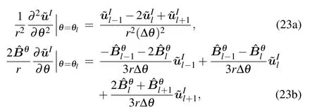
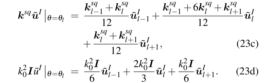
The azimuth angle period is 2π. As a result,the periodic boundary condition is applied in the azimuth angle direction,forming a closed-form matrix equation. For simplicity,we can choose an angle where the environmental parameters do not change or vary slowly at the start and end computation points because only the coupling along therdirection should be considered. Then, substituting Eq. (23) into Eq. (22b), we can obtain a tridiagonal matrix for the ease of recurrence calculations.
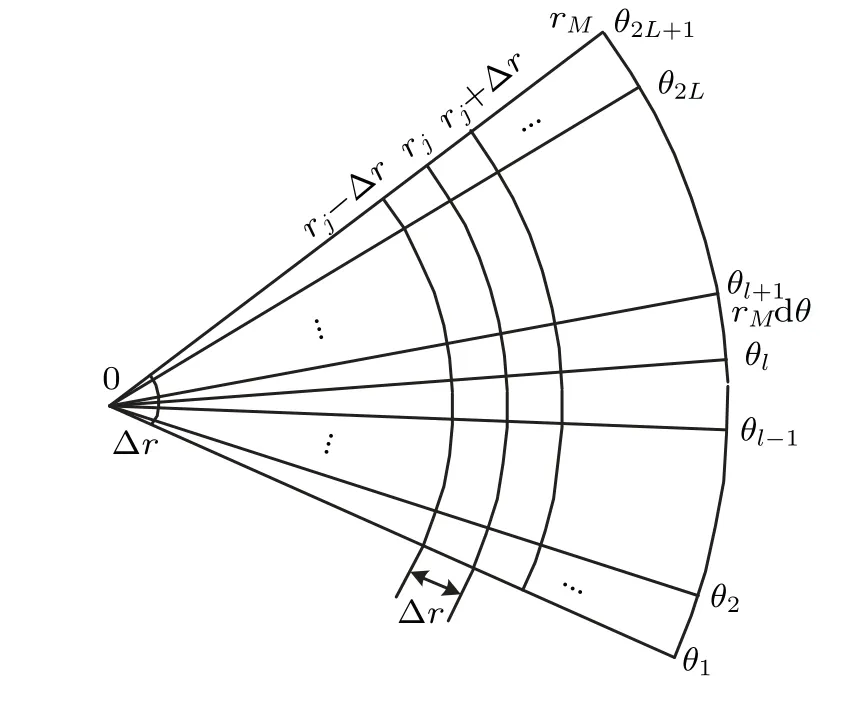
Fig.2. Discretization of the horizontal plane.
3. Model verification
3.1. Accuracy of the numerical implementation
In order to test the accuracy of the numerical implementation,we use the 3D coupled-mode model to compute a rangeindependent waveguide case,which is shown in Fig.3,and the results are compared with those obtained by using the FT-CM model.[17]
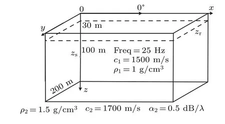
Fig.3. Range-independent waveguide.
Although this case does not involve coupling, it is sufficient for the accuracy of the model’s numerical implementation. This range-independent waveguide consists of a homogeneous water column with a sound speed of 1500 m/s, a density of 1 g/cm3, and a water depth of 200 m. It is limited above by a pressure-release sea surface and below by a homogeneous fluid half-space bottom with a sound speed of 1700 m/s,a density of 1.5 g/cm3,and attenuation of 0.5 dB/λ.A point source is located 100 m in the depth direction,and the source frequency is 25 Hz. Moreover,the receiver depth considered is 30 m, and the transmission loss (TL) computed by the two models is shown in Figs.4 and 5.

Fig.4. Comparison of TLs at a 0?angle and 30 m depth in the rangeindependent waveguide computed by the presented and FT-CM models.

Fig.5. The horizontal distribution of acoustic field at a depth of 30 m for a range-independent waveguide. The left panel is computed by the FT-CM model,and the right panel is computed by the 3D CM model.
The close agreement between the two models clearly demonstrates that the numerical implementation is accurate for 3D acoustic calculations. We can obtain a sufficient azimuth angle range to satisfy the computation requirement based on the high-order Pad′e approximation and the split-step method. Meanwhile,the circular interference structure can be presented on the horizontal plane due to the interference of different modes in the range-independent waveguide.
3.2. Accuracy of mode coupling
In order to verify the accuracy of mode coupling in the 3D model, a wedge waveguide is considered. Although the waveguide is a simpler case, it has a topographical variation along the bearing angle and the radial direction. This wedge waveguide consists of a water column with a sound speed of 1500 m/s and a density of 1 g/cm3. It is limited above by a pressure-release sea surface and below by a fluid half-space bottom with a sound speed of 1700 m/s,a density of 1.5 g/cm3,and attenuation of 0.5 dB/λ.A point source is located 100 m in depth,and the source frequency is 25 Hz. The receiver depth considered is 30 m. For the up-sloping wedge with 2.86?,as shown in Fig. 6, the 3D acoustic fields are computed and shown in Figs. 7 and 8. Moreover, the down-sloping wedge waveguide,as shown in Fig.9,is under consideration,and the result is shown in Figs.10 and 11.
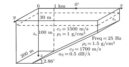
Fig.6. The geometry of an up-sloping wedge waveguide.
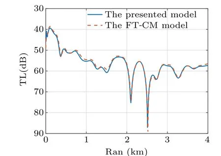
Fig.7. Comparison of TLs at a 0?angle and 30 m depth in the up-sloping wedge waveguide computed by the presented and FT-CM models.
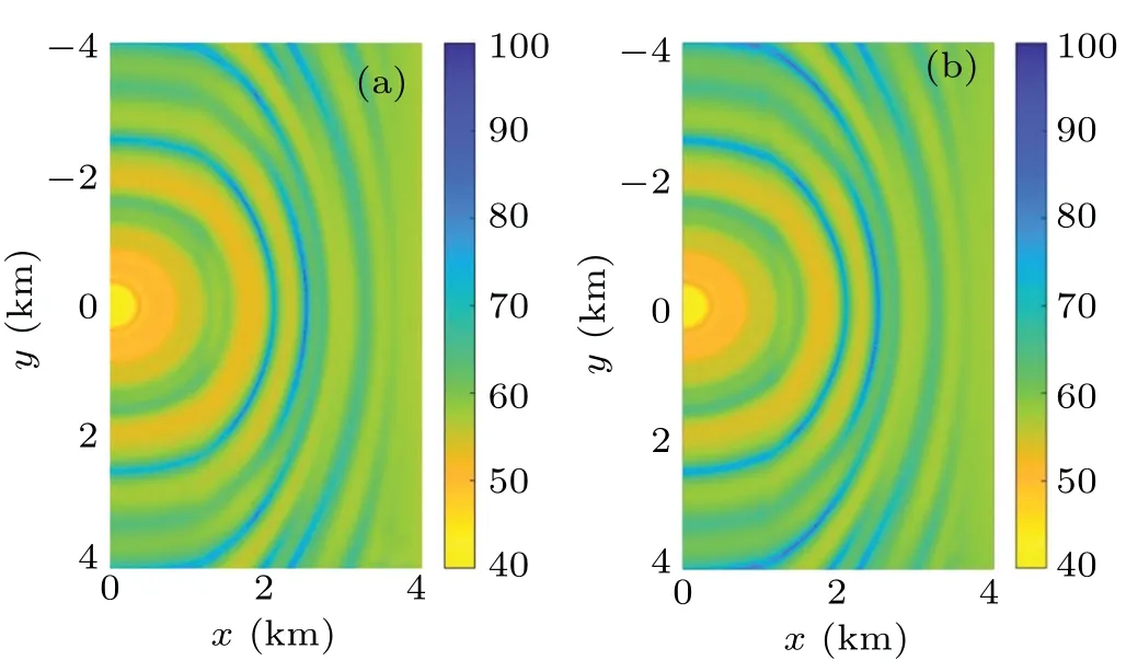
Fig.8. The horizontal distribution of acoustic field at a depth of 30 m for the up-sloping wedge. The left panel is computed by the FT-CM model,and the right panel is computed by the 3D CM model.
The simulation results show that the two model’s close agreement demonstrates that mode coupling can be effectively handled in this 3D coupled-mode model. Although a slight difference is evident from Figs.7 and 10 because the treatment of the mode coupling varies.Therefore,the error is acceptable.Meanwhile, the horizontal interference structure also varies with the topography because the acoustic field energy moves toward the direction where the ocean depth increases.The horizontal interference structure diverges into elliptic rings with the increase in the ocean depth. The interference structure forms compressed ellipses when the ocean depth decreases.
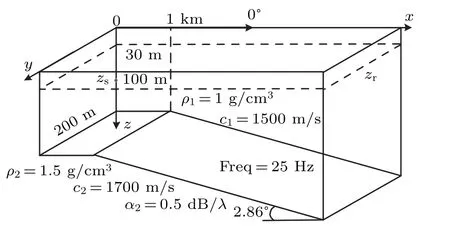
Fig.9. The geometry of a down-sloping wedge waveguide.
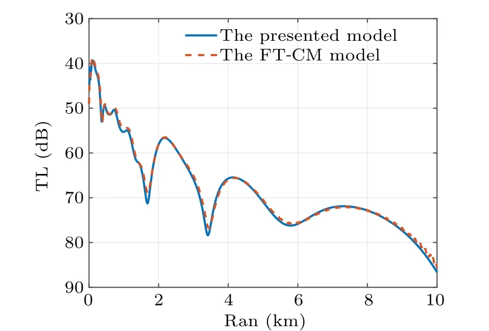
Fig. 10. The comparison of TLs at a 0?angle and 30 m depth in the down-sloping wedge waveguide is computed by the presented and FTCM models.
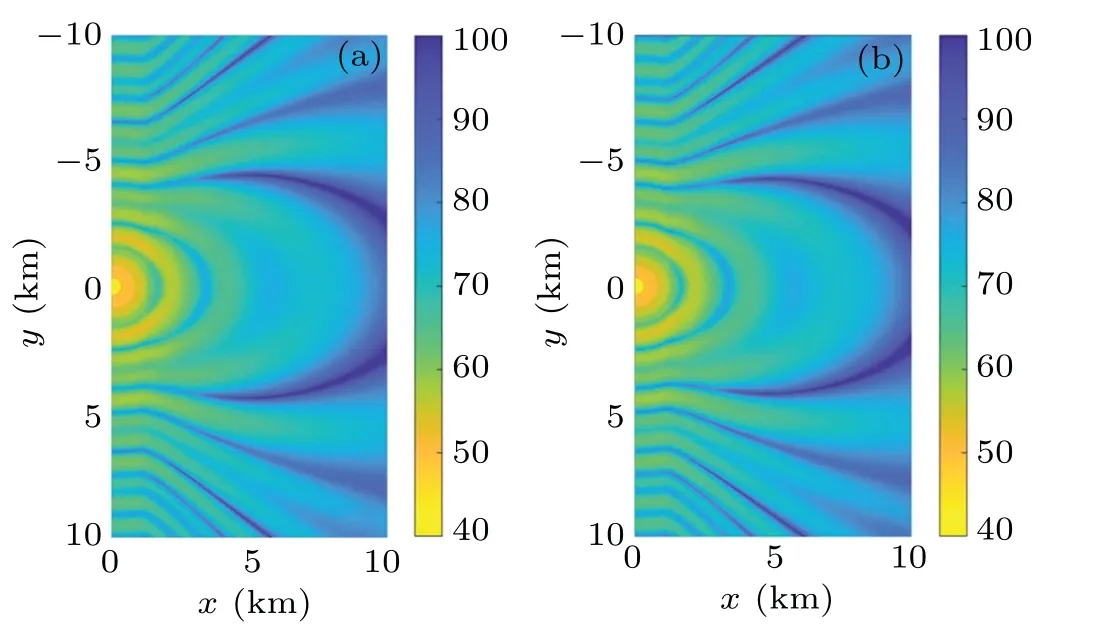
Fig. 11. The horizontal distribution of the acoustic field at a depth of 30 m for the down-sloping wedge. The left panel is computed by the FT-CM model,and the right panel is computed by the 3D CM model.
3.3. Range of azimuth angle calculation
Based on the split-step method and high-order Pad′e approximation, the 3D coupled-mode model in this paper has a highly wide-angle azimuth range. For the high-order Pad′e square root approximation,the accurate of the angle has been effectively analyzed in parabolic equation.[20,21]In order to verify the accuracy of the azimuth angle calculation range in the 3D model in this study,a conical seamount waveguide case is considered,as shown in Fig.12. This seamount waveguide consists of a water column with a sound speed of 1500 m/s and a density of 1 g/cm3. It is limited above by a pressurerelease sea surface and below by a fluid half-space bottom with a sound speed of 1700 m/s,a density of 1.5 g/cm3,and attenuation of 0.5 dB/λ. The height of the seamount is 100 m,and the radius of the seamount base is 2 km. A point source is located 100 m in depth, and the source frequency is 25 Hz.Additionally,the receiver depth considered is 30 m.

Fig.12. The seamount waveguide for azimuth angle analysis.
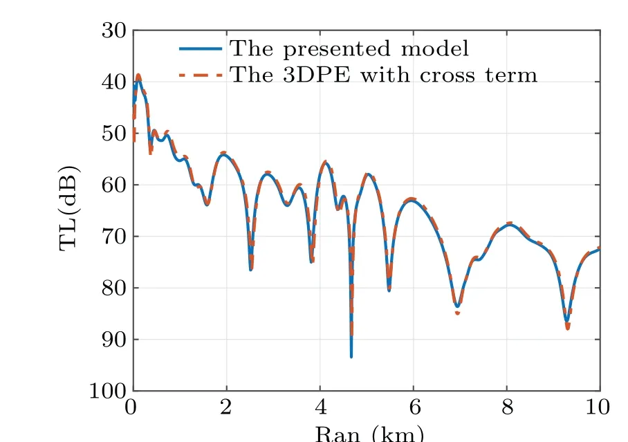
Fig. 13. The comparison of TLs at a 0?angle and 30 m depth in the conical seamount waveguide is computed by the presented and 3D PE models.
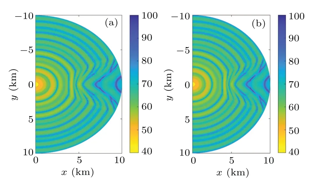
Fig. 14. The horizontal distribution of the acoustic field at a depth of 30 m for the down-sloping wedge. The left panel is computed by the 3D PE model with the cross-term, and the right panel is computed by the 3D CM model.
As a comparison of the 3D coupled model,a 3D parabolic equation method and the square root approximation with the cross-term is used.[5,6,8]This cross-term approximation method has a high calculation precision on the azimuth of[?90?,90?]. The TL computed by the two models is shown in Figs.13 and 14.
The agreement between the two models signifies that the numerical implementation is accurate on the wide azimuth angle range. However,a difference is evident because these two models substantially vary in theory and numerical implementation. For the coupled model, the accurate solution of the local eigenvalue and eigenfunction is still a key issue and generates an error. For the parabolic equation, the operator expansion with the cross-term is equivalent to the second-order Taylor series and only partially increases the calculation precision. The truncation of the cross-term also introduces an error in the numerical implementation. Therefore, this difference is inevitable. Meanwhile,from the mathematical perspective,compared with the second-order Taylor series of the square root included two horizontal coordinates,the high-order Pad′e approximation of the azimuth square root has more precision on the azimuth.
4. Effect on acoustic field caused by seamount
4.1. Effect of the seamount size
The seamount size obviously affects the low-frequency acoustic field in the waveguide. In order to analyze the extent of the effects of the seamount size on sound propagation,various conical seamounts sizes are considered, as illustrated in Fig.15. The height of the seamountHm,and the radius of the base of the seamountRmare(150 m,500 m),(150 m,200 m),and (100 m, 500 m). This seamount waveguide consists of a water column with a sound speed of 1500 m/s and a density of 1 g/cm3. It is limited above by a pressure-release sea surface and below by a fluid half-space bottom with a sound speed of 1700 m/s,a density of 1.5 g/cm3,and attenuation of 0.5 dB/λ.Based on the presented 3D CM model,the TLs are computed and shown in Fig. 16, and the horizontal distributions of the acoustic field at a depth of 30 m are shown in Fig.17.
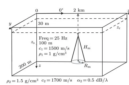
Fig.15. Geometry of the ideal seamount problem.
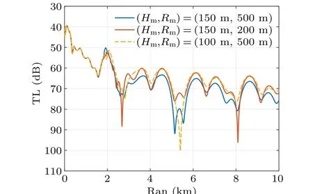
Fig. 16. Comparison of TLs at 0?azimuth angle and 30 m depth in waveguides with seamounts of different sizes.
It can be seen from the calculation results that the acoustic field after the seamount in case (a) is not only lower by about 5 dB than the others but also has a larger interference anomaly region. From the perspective of mode coupling, the radius of the seamount influences the coupling range of the normal modes, and the height of the seamount impacts the normal mode types. When the radius is larger,the mode coupling between the area after the seamount and the no seamount affected area is weaker, causing the anomaly acoustic field recovery to be challenging after the seamount. Meanwhile,the normal mode can be classified into the trapped and leaky modes according to the critical grazing angle.The seamount is high,and there are few normal trapped modes. There are two normal trapped modes in a 100 m height seamount waveguide mountaintop,whereas only one trapped normal mode exists in a 150 m height seamount waveguide mountaintop.Though the energy tends to be stored in the waveguide because of mode coupling,the leaky modes increase the energy losses.

Fig.17. Horizontal distribution of acoustic field at a depth of 30 m in the waveguides with seamounts of height and radius(a)(150 m,500 m),(b)(150 m,200 m),and(c)(100 m,500 m).
4.2. Mode coupling caused by seamount
In order to analyze the mode coupling effect caused by the seamount, the acoustic fields are computed by the adiabaticN×2Dand 3D CM methods by ignoring or considering all the mode couplings in a seamount waveguide. The height of the seamount is 150 m,the radius is 500 m,and all other environmental parameters are the same as those of the waveguide shown in Fig. 15. The horizontal distribution of the acoustic field at a 30 m depth is shown in Fig.18.
As shown in Fig. 18, the anomaly region of the acoustic field computed by the 3D model is more significant than that by the adiabaticN×2Dmodel. The adiabaticN×2Dmodel cannot embody the horizontal refraction phenomenon,meaning that the horizontal refraction caused by the seamount exists. Meanwhile,the energy after the seamount is calculated by the 3D CM method by considering that the entire coupling effect is greater than those of the other two, and the interference structure tends to recover in the waveguide without the seamount. This suggests that the low-frequency acoustic field can diffract to a certain extent through the seamount.
According to mode coupling theory and parabolic coupled mode of Eq.(13),these two phenomena are not difficult to explain. The energy transformation between modes,which is indicated by the radial coupling term,tends to limit the energy in the waveguide.Meanwhile,the acoustic field reverts to the situation without the seamount owing to the azimuth coupling behind the seamount and other directions.Except for the azimuth coupling term,the other terms in the square illustrate that the horizontal energy propagates toward the increased ocean depth, which is called horizontal refraction. This term is ignored in theN×2Dmethod.
In order to analyze the mode coupling and 3D acoustic field caused by the topography and to eliminate the effects of the source and receiver location,we define the relative amplitude of the normal mode as
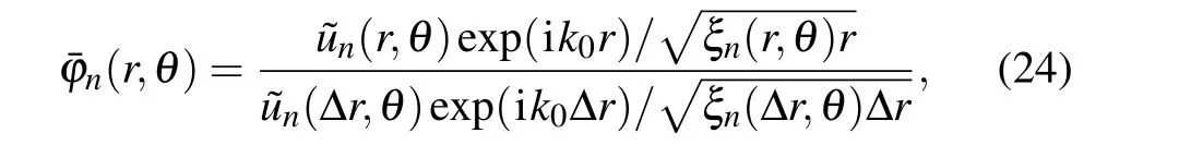
where ?ris the range interval in computation. For the case depicted in Fig.18,the distributions of the relative amplitudesˉ?n(r,θ)of the first four orders of normal modes are shown in Fig.19.

Fig.18. Horizontal distribution of acoustic field at a depth of 30 m in the waveguides with seamounts of height and radius(150 m,500 m): (a)adiabatic N×2D model;(b)3D CM method that ignores all the mode coupling;(c)3D CM method that considers all the mode coupling.

Fig.19. Relative amplitudes of the normal modes: (a)first-order,(b)second-order,(c)third-order,and(d)fourth-order.
The distribution of the local eigenvalues illustrates that at the starting range where the ocean depth is 200 m, the first three modes are trapped normal modes, and the fourth-order mode is the leaky mode. At a range of 2 km,where the mountaintop is 50 m from the ocean surface, only the first-order mode is the trapped normal mode, and the rest are the leaky normal modes. The relative amplitudes of the normal modes after the seamount propagates toward the deeper area form a radiative area after the seamount. Further,dark and bright radial interference patterns can be seen because of mode coupling,as shown in Fig.19.
The first-order mode is the trapped constant normal mode,but the relative amplitude differs before and after the seamount due to the propagation deflection and mode coupling.The second and third modes form a circular weak energy area at the center of the seamount because of the cutoff of the trapped normal modes.Furthermore,the fourth-order mode is the constant leaky mode,and its energy theoretically leaks to the bottom.However,there is a noticeable energy distribution change at the seamount,as shown in Fig.19(d). This change happens at the depth where the third-order mode transforms into the leaky mode from the trapped mode.
5. Conclusions
A three-dimensional coupled-mode (3D CM) model is built for waveguides with arbitrary topographies to compute the acoustic fields under restricted nonhorizontal boundary conditions. In the process of modeling, the couplings along the radial and azimuthal directions are effectively considered by the operator theory and high-order rational approximations.Further, the 3D CM method is easy to implement numerically and can solve the wide-angle sound propagation problem. This method has the advantages of the coupling mode and parabolic equation theory. By simulating in the rangeindependent waveguide,the wedge waveguide,and the conical seamount waveguide, the accuracy of the 3D CM model can be demonstrated,and the results illustrate that this model can effectively estimate the horizontal refraction and couplings along the horizontal direction.
From the view of mode coupling, the low-frequency 3D sound propagation phenomena caused by the seamount are discussed based on the 3D CM model. The results indicate that the topographical changes can cause the acoustic field to deflect toward the direction of increase of the ocean depth,and the mode coupling occurs along the horizontal direction of the topographical variation. The deflection of the acoustic field causes horizontal refraction and a fan-shaped abnormal acoustic field area after the seamount. While mode coupling occurs along the radial and azimuth angle directions,the energy tends to be stored in the waveguide and propagates by diffraction past the seamount. The influence of the seamount on the lowfrequency acoustic field is related to the height and radius of the seamount. The height of the seamount limits the number of the trapped normal modes, and the radius of the seamount dictates the scope of the coupling effect. The larger the mountain(the seamount is higher and has a larger radius),the more the effect of the seamount on the acoustic field. In conclusion, the complex waveguide with a seamount cannot ignore the out-of-plane effects and mode coupling. The horizontal refraction increases the influence area of the seamount,but the diffraction from mode coupling weakens the total influence of the seamount.
Acknowledgements
Project supported by the National Natural Science Foundation of China (Grant No. 11804360), the IACAS Frontier Exploration Project (Grant No. QYTS202103), and the Key Laboratory Foundation of Acoustic Science and Technology(Grant No.2021-JCJQ-LB-066-08).

- Chinese Physics B的其它文章
- Magnetic properties of oxides and silicon single crystals
- Non-universal Fermi polaron in quasi two-dimensional quantum gases
- Purification in entanglement distribution with deep quantum neural network
- New insight into the mechanism of DNA polymerase I revealed by single-molecule FRET studies of Klenow fragment
- A 4×4 metal-semiconductor-metal rectangular deep-ultraviolet detector array of Ga2O3 photoconductor with high photo response
- Wake-up effect in Hf0.4Zr0.6O2 ferroelectric thin-film capacitors under a cycling electric field