Dynamic Analysis of Launch Vehicle Piping Systems

WANG Shuai ,LI Chao ,ZHOU Yuguo ,ZHANG Xinyao ,YANG Dongsheng ,ZHONG Sheng

1 Aerospace System Engineering Shanghai,Shanghai 201109

2 Xichang Satellite Launch Center,Xichang 615600

Abstract: Due to complex assembly boundaries and working environment of the piping system in a launch vehicle,it is difficult to simulate realistic flight conditions on the ground.The lack of analysis on the complex environment and boundary conditions in the design process may lead to flight failures,even cause the fuel to combust and destroy the launch vehicle.This paper studies the technology and methods for dynamic simulation analysis of piping systems in launch vehicles,and established a dynamic simulation model of representative pipelines,which is expected to provide a basis for simulation analysis of piping system states in realistic flight.

Key words: launch vehicle,piping system,dynamic strength,simulation

1 INTRODUCTION

As a channel connecting tanks and engines,the piping system of a new-generation launch vehicle plays an important role in the flight phase of the launch vehicle.The piping system contains compensators,curved pipes,straight pipes,flanges and brackets,and features complex assembly boundaries and operating environment[1].Any leakage or fracture of the piping system during launch preparation and in flight may lead to combustion and explosion of the launch vehicle,causing possible fatalities and enormous economic loss[2].

The integrity of the piping system design is tested by ground testing,which cannot provide a truly representative flight environment due to constraints.Thus,effective methods for dynamic simulation analysis of complex environment and boundaries are necessary[3].Poor quality of large-diameter cryogenic piping systems is usually caused by lack of recognition of complex environment and boundary conditions which piping systems would experience in the design process[4].

In this paper,we study dynamic simulation modeling methods for piping systems in launch vehicles and methods for finite element analysis,and then establish a simulation model of representative piping systems in launch vehicles and conduct strength and fatigue analyses.We also offer a prospect on the following research and analysis[5].

2 RESEARCH ON DYNAMIC ANALYSIS OF PIPING SYSTEMS

For conducting strength analysis of a typical piping system composed of components including compensators,curved pipes,straight pipes,flanges and brackets,the very first step is to establish geometric and material models based on the the piping system components,layout and installation and specify the boundary conditions and constraints.The assembly of the piping system is shown in Figure 1.The next step is modeling for analysis,which includes the mechanical properties of pipes,brackets and compensators.Finally,an equivalent mechanical model is established with appropriate settings of boundary conditions and modeling of key parts (like brackets and compensators),so the simulation model of piping systems will satisfy the engineering design requirement.

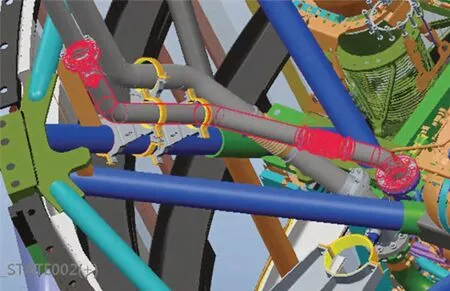
Figure 1 Assembly of the piping system

2.1 Geometric Models

Based on real assembly conditions,a 3-dimension model for the piping system is used as the geometric model for finite element analysis[6],as shown in Figure 2.The piping system is fixed on the engine frame by holders,with its top end connected to outer systems and bottom connected to the engine by the top flange and bottom flange,respectively.

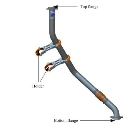
Figure 2 Geometric model of a piping system

2.2 Material Models

1Cr18Ni9Ti is selected as the material for pipes and compensators,its major properties are shown in Table 1.

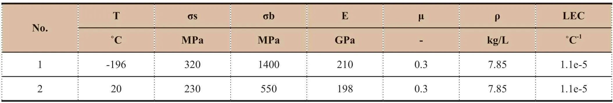
Table 1 Material property parameters

2.3 Boundary Conditions

Large regional stress may occur in the constraint areas,due to temperature loading and forced displacement boundary conditions during the loading process.To solve the problem,extending the upper part of the pipe appropriately,and using the extended part as tie constraint with the original constraint,so to ensure the new constraint would not impact the dynamics of the whole structure[7].

2.4 Constraint Processing

The top and bottom flanges of a piping system are clamped in 6 degrees of freedom (set reference points,which is interconnected with flanges,as clamped);set a reference point at the central point of the holder,which is the assembly position in the pipe,then connect the reference point and the holder,and finally clamp the degrees of freedom of X,RX,RY[8].The constraint conditions of a pipe is shown in Figure 3.

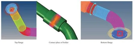
Figure 3 Constraint conditions of a pipe

2.5 Equivalent Model for Compensators

Compensator modeling adopts the approximate stiffness method (as shown in Figure 4).During the modeling process,the compensator structure is simplified as a double-layer corrugated pipe,and the outer layer is bound with the inner layer at the adjacent nodes,in order to realize synchronous motion in two layers.The outer layer nodes are bound with the neighboring nodes of the inner layer[9].

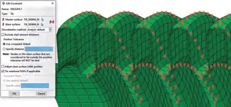
Figure 4 Compensator modeling method

2.6 Equivalent Model for Holders

Holders are simplified as shell units.The “softer” entity units are filled between holders and pipes,in order to “loosen”strong coupling induced damping.The elastic modulus of the entity is set as one tenth of a percent of the pipe material,and it shares the same nodes with shell units[10].The holder modeling method is shown in Figure 5.

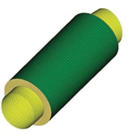
Figure 5 Holder modeling method

2.7 Finite Element Modeling

The main structure of the piping system is considered a shell.This makes the pipe model discrete by using a linear fully integrated element.There are 62375 nodes and 58717 units in the finite element (FE) model,the types used in the element are S4 and C3D8R.The FE model is shown in Figure 6[11].

Figure 6 Finite element model for piping system

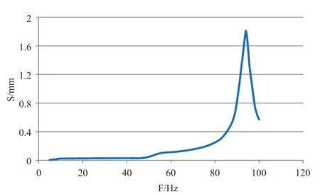
Figure 7 The frequency related response of displacement with X direction excitation

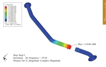
Figure 8 Total displacement of pipes

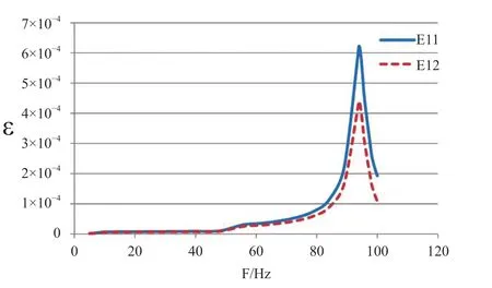
Figure 9 The frequency related response of strain with X direction excitation

3 DYNAMICS SIMULATION ANALYSIS OF PIPING SYSTEMS

Assumptions of the FE model of the piping system:

1) Gravity;

2) Set inner fluid is liquid oxygen,under the loading pressure of 2 MPa;

3) The temperature is -183°C.

3.1 Simulation Analysis of Sine Sweep Response

3.1.1 Loading

Loading of sine sweep is shown in Table 2,where the displacement excitation for 5 -10 Hz is replaced as a corresponding acceleration.

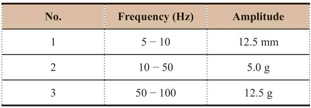
Table 2 Sine sweep loading

3.1.2 Results of Simulation Analysis

The frequency related responses of displacement and strain under the excitation in X direction are shown in Figures 7,8 and 9.When the excitation frequency is 93.9 Hz,the largest regional displacement occurs,as 1.81 mm,and the strain reaches the largest level,as axial strain of 621με,and circumferential strain of 432με,as shown in Figure 10.

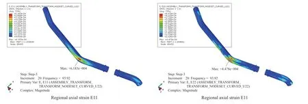
Figure 10 Regional largest strain of pipes with the excitation of 93.9 Hz in X direction

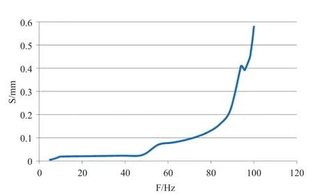
Figure 11 The frequency related response of displacement with Y direction excitation

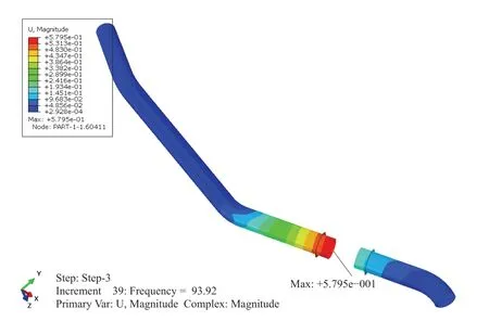
Figure 12 Total displacement of pipe

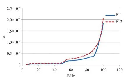
Figure 13 The frequency related response of strain with Y direction excitation

The frequency related responses of displacement and strain under the excitation in Y direction are shown in Figures 11,12,13.When the excitation frequency is 100 Hz,the largest regional displacement occurs as 0.58 mm,as shown in Figure 14.The strain almost reaches the second order natural frequency when the excitation in Y direction is up to the upper band 100 Hz.Therefore,it is close to resonation with the largest amplitude response.The strain also reaches the largest with an axial strain of 182με,and circumferential strain of 204με.

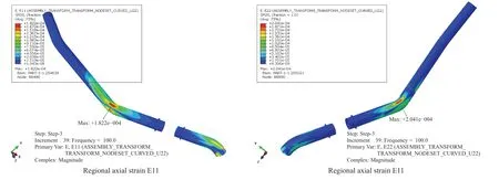
Figure 14 Regional largest strain of pipes with the excitation of 100 Hz in Y direction

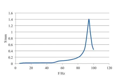
Figure 15 The frequency related response of displacement with Y direction excitation

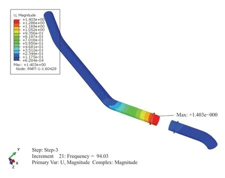
Figure 16 Total displacement of pipes

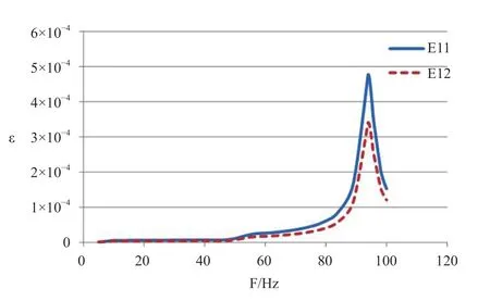
Figure 17 The frequency related response of strain with Z direction excitation

The frequency related responses of displacement and strain under the excitation in Z direction are shown in Figures 15,16,17.When the excitation frequency is 94.0 Hz,the largest regional displacement occurs as 1.40 mm,and the strain reaches the largest level,with an axial strain of 479με,and circumferential strain of 346με,as shown in Figure 18.

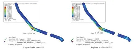
Figure 18 Regional largest strain of pipes with the excitation of 82.27 Hz in Z direction

3.2 Random Vibration Simulation Analysis

3.2.1 Loading

The selected power spectral density is shown in Table 3.

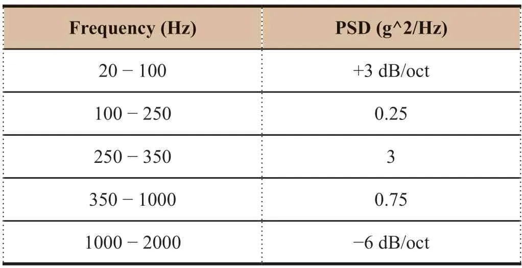
Table 3 Power spectral density

3.2.2 Results of simulation analysis

Root-Mean-Square (RMS) displacement and acceleration in X direction are shown in Figure 19,the largest regional axial strain is 548με,and the largest circumferential strain is 521με.

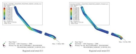
Figure 19 RMS strain (X)

RMS displacement and acceleration in Y direction are shown in Figure 20,the largest regional axial strain is 504με,and the largest circumferential strain is 599με.

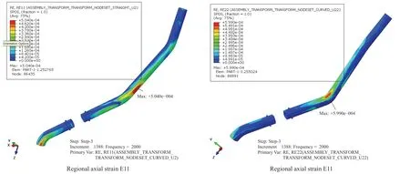
Figure 20 RMS Strain(Y)

RMS displacement and acceleration in Z direction are shown in Figure 21,the largest regional axial strain is 348με,and the largest circumferential strain is 402με.

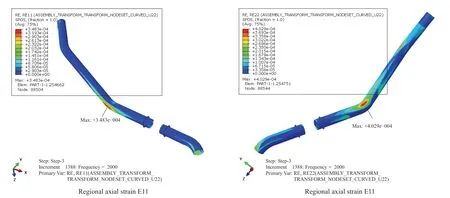
Figure 21 RMS strain (Z)

4 FATIGUE ANALYSIS FOR PIPING SYSTEMS

4.1 Fatigue Analysis Methods for Piping Systems

First,we performed a sweep frequency analysis of pipeing systems,which was input of a frequency response analysis requested in fatigue analysis settings.As the static compensation,the static analysis would affect the fatigue life depending on the average stress.Next,we created a vibration loading spectrum using a random,sweep frequency,and conducted a specific frequency fatigue analysis.Then,we created the Mises stress-power spectrum curve of structures under the random vibration.The fatigue life under the random vibration could be calculated based on the Dirlik method combined with Miner linear accumulated damage theory.Lastly,we created the cloud figure of fatigue analysis,and chose the node with the largest potential damage as the risk node for fatigue analysis[12].The fatigue analysis process is shown in Figure 22.

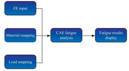
Figure 22 Fatigue analysis process

Fatigue strength test was assessed mainly by the damage to the structures.Damage is the derivative of fatigue life:

The damage caused in one cycle equals to1/Nf,where theNfmeans the cycle during which structure failed under a specific stress level.Thus,under the stressi,the total damage equals the period of loading stress n by failure periodN.

All directions were evaluated for damage during the test of fatigue strength.The qualified condition was that damage should be less than 0.1 in a certain direction.

4.2 Simulation Results of Piping Systems

Analyzing the fatigue simulation for the piping system using nCode and ABAQUS,after settings of random vibration,sweep frequency spectrum,specific frequency spectrum,material curve,analysis of response file (OBJ),the prestress analysis result file (ODB) were completed.In addition,the prestress effect should be considered under real conditions.It is transformed as average stress in the fatigue analysis.The prestress effect should not be considered in the result of sweep frequency,otherwise,it would be contained in special socket data,and would be corrected using Goodman Average Stress Correctness Method.

4.2.1 Random fatigue analysis results

The lowest life is 1.626E+05 s under random vibration in X direction.In the case of 300 s testing time,the equivalent damage is 1.85E-03.The position of the highest damage risk is at the connection between the desuperheating pipe and the engine.The cloud figures of life and damage under random vibration in X direction are shown in Figure 23 and Figure 24,respectively.

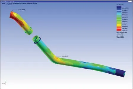
Figure 23 Cloud figure of life under random vibration in X direction

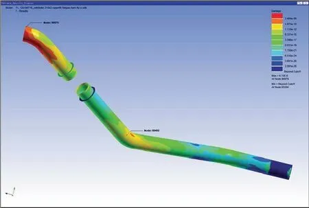
Figure 24 Cloud figure of damage under random vibration in X direction

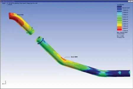
Figure 25 Cloud figure of life under random vibration in Y direction

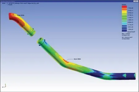
Figure 26 Cloud figure of damage under random vibration in Y direction

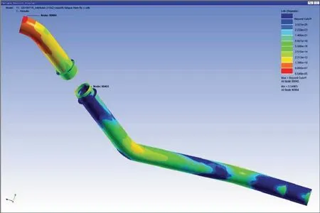
Figure 27 Cloud figure of life under random vibration in Z direction

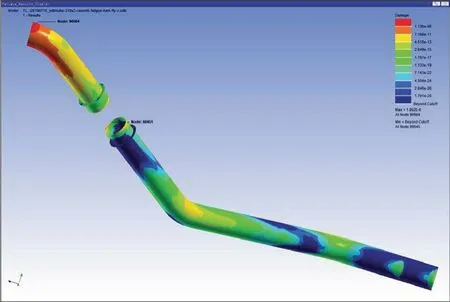
Figure 28 Cloud figure of damage under random vibration in Z direction

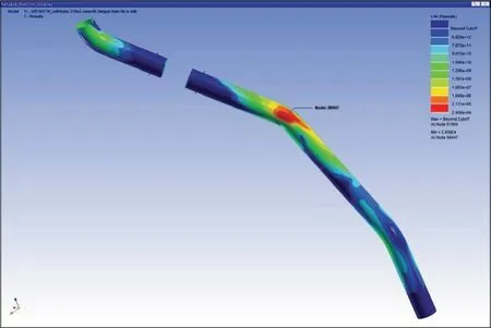
Figure 29 Cloud figure of life under sweep frequency vibration in X direction

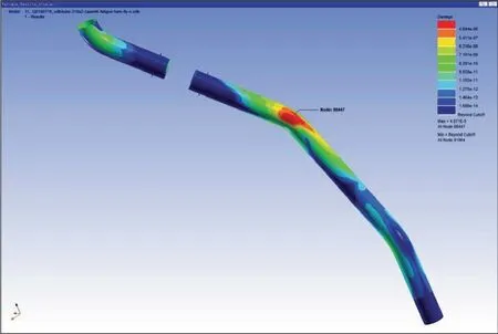
Figure 30 Cloud figure of damage under sweep frequency vibration in X direction

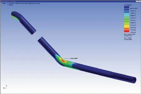
Figure 31 Cloud figure of life under sweep frequency vibration in Y direction

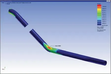
Figure 32 Cloud figure of damage under sweep frequency vibration in Y direction

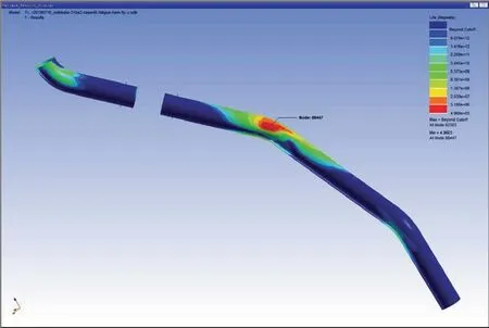
Figure 33 Cloud figure of life under sweep frequency vibration in Z direction

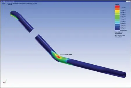
Figure 34 Cloud figure of damage under sweep frequency vibration in Z direction

The lowest life of structures is 5.336E+05 s under the random vibration in Y direction.In the case of 300 s testing time,the equivalent damage is 5.62E-04.The highest risk position for damage is at the connection position with the engine.The cloud figures of life and under random vibration in Y direction damage are shown in Figures 25 and 26,respectively.

The lowest life is 5.55E+05 s under the random vibration in Z direction,the equivalent damage is 5.40E-04.The highest risk position for damage is at the connection position with the engine.The cloud figures of life and damage under random vibration in Z direction are shown in Figures 27 and 28,respectively.

4.2.2 Sweep frequency analysis results

The lowest life for fatigue is 2.46E+04 times,under the sweep frequency vibration in X direction.The most hazardous part is at the curve in the middle of desuperheating pipe.The cloud figures of life and damage under sweep frequency vibration in X direction are shown in Figures 29 and 30,respectively.

The lowest life for fatigue is 1.88E+08 times,under the sweep frequency vibration in Y direction.The most hazardous part is at the curve in the middle of desuperheating pipe,as shown in Figures 31 and 32.

The lowest life for fatigue is 4.96E+05 times,under the sweep frequency vibration in Z direction.The most hazardous part is at the curve in the middle of desuperheating pipe,as shown in Figures 33 and 34.

5 CONCLUSION AND PROSPECTS

This paper studies the method of dynamic strength modeling for simulation analysis of a piping system,which is suitable for analysis of complex environment and boundary conditions of the system.The strength simulation analysis and fatigue simulation analysis were performed based on the established model for piping system dynamic strength simulation.The simulation results show the effectiveness and correctness of the model and analysis method.In the future,experiments could be carried out for key materials and structures,to test the properties under super cold temperatures and fatigue.The fatigue life curve could be obtained by experiment under normal and super cold temperatures.We will further optimize finite element analysis and specific algorithms,develop fatigue design criteria for piping systems,and fatigue life and reliability evaluation methods,providing guidelines for design optimization of piping systems.