INTERFACE BEHAVIOR AND DECAY RATES OF COMPRESSIBLE NAVIER-STOKES SYSTEM WITH DENSITY-DEPENDENT VISCOSITY AND A VACUUM*

(郭真華) (張學(xué)耀)

1. School of Mathematics and CNS, Northwest University, Xi’an 710127, China;

2. School of Mathematics and Information Science, Guangxi University, Nanning 530004, China E-mail: zhguo@gxu.edu.cn; xyzhang05@163.com

Abstract In this paper,we study the one-dimensional motion of viscous gas near a vacuum,with the gas connecting to a vacuum state with a jump in density.The interface behavior,the pointwise decay rates of the density function and the expanding rates of the interface are obtained with the viscosity coefficient μ(ρ) = ρα for any 0 ＜α ＜1; this includes the timeweighted boundedness from below and above.The smoothness of the solution is discussed.Moreover,we construct a class of self-similar classical solutions which exhibit some interesting properties, such as optimal estimates.The present paper extends the results in [Luo T, Xin Z P, Yang T.SIAM J Math Anal, 2000, 31(6): 1175-1191] to the jump boundary conditions case with density-dependent viscosity.

Key words decay rates; interface; Navier-Stokes equations; vacuum

1 Introduction

We consider the one-dimensional compressible Navier-Stokes equations for isentropic flows in Eulerian coordinates

wherex ∈R,t ＞0, andρ=ρ(x,t),u=u(x,t) andP(ρ) denote, respectively, the density, the velocity and the pressure;μ(ρ) =ραis the viscosity coefficient which is possibly degenerate,andα ＞0 is a constant.For simplicity, we consider only a polytropic gas withP(ρ) =ργ,γ ＞1.

There have been many works considering the global existence and large-time behavior of solutions to (1.1) (a complete review of the literature on this is far beyond the scope of this paer).With one boundary fixed and the other connected to a vacuum, Okada, in [22], proved the global existence of the weak solution to the free boundary problem of(1.1)for the constant viscosity case.Similar results were obtained by Okada and Makino in [23] for the equations of the spherically symmetric motion of viscous gases.Further understanding of the regularity and the behavior of solutions near the interfaces between the gas and the vacuum was provided by [17].In what follows, we shall focus on some closely relevant works, considering the onedimensional problem in free boundary settings with density-dependent viscosity.For when the initial density connects to a vacuum with discontinuities, see [5, 13, 14, 18, 19, 21, 24, 29, 34]and the references therein.For when the initial density is assumed to be connected to a vacuum continuously, please refer to [1, 2, 6, 7, 25, 28, 33] and the references therein.

Concerning the asymptotic behavior of the weak solution to (1.1) where the initial density connects to a vacuum continuously, and under the transformation in Lagrangian coordinates

In the present paper, certain decay rates of the density function and expanding rates of the free boundary with respect to time are obtained for any 0＜α ＜1,γ ＞1; these include, in particular, the time-weighted boundedness from below and above.Based on these, we can be assured that the density function tends to zero and that the volume of the gas domain tends to infinity at an algebraic rate as the time tends to infinity.Moreover, we obtain a better timeweighted upper bound of the density function compared with [6, 7, 34].To obtain the lower bound of the density, an estimate on the derivative of the density function is necessary; that is,withk=1 asγ ≥1+α,andk=nas 1＜γ ＜1+α,which,together with, gives the time-weighted lower bound of the density by the method from [14].In addition, for any 0＜α ＜1,γ ＞1+2α, by establishing some uniform time-weighted estimates to (ρ,u), a sufficient condition on the lower bound of the density function for ensuring that the optimal decay of the density holds is given.Finally,we construct the exact self-similar classical solution to the free boundary problem of (1.1).It is shown that this class of solutions exhibits some important elements, including more explicit regularities, the large-time behavior of both the density and the velocity on the free boundary,and the optimal estimates of the solution and the gas domain.

Throughout this paper, we assume that the entire gas initially occupies a finite interval[a,b]?R, and connects to a vacuum discontinuously.The assumptions on the initial data are stated as follows:

(A1)ρ0(x)＞0,?x ∈[a,b];ρ0(x)∈W1,∞([a,b]);

(A2)u0(x)∈H1([a,b]).

If the support of the density function is compact,then there exist two curves,a(t)andb(t),issuing initially fromaandb, respectively, separating the gas and the vacuum; that is,

witha(0)=aandb(0)=b.

We consider the free boundary problem (1.1) in (x,t)∈（a(t),b(t)）×(0,+∞), imposing with the jump boundary conditions and initial data

whereP(ρ)=ργ(γ ＞1),μ(ρ)=ρα(α ＞0).

The definition of a weak solution to (1.2) is given below.

Definition 1.1(ρ,u)is called a weak solution to the free boundary problem(1.2)if there exista(t) andb(t)∈C([0,+∞)) such that

hold for anyφ ∈C10(Ω) with Ω={(x,t)|a(t)≤x ≤b(t),0≤t ＜+∞}.

In what follows,Ci(i=0,1,···,6)denote some positive constants independent oftandx.

We now state our first result, which gives the existence and asymptotic behavior of the weak solution of problem (1.2).

Theorem 1.2Letρ0andu0satisfy (A1)-(A2), 0＜α ＜1.Then the free boundary problem (1.2) has a unique global weak solution (ρ,u) witha(·),b(·)∈C1([0,+∞)) satisfying that

(i) for any 0＜η ?1,

The next theorem shows the smoothness of the solution obtained in Theorem 1.2 under the appropriate initial regularity.

Theorem 1.6Let (ρ,u) be the weak solution to (1.2) described in Theorem 1.2.If(ρ0xx,u0xx)∈L2([a,b]), then

Remark 1.8The self-similar solution in Theorem 1.7 possesses a great deal of interesting information, including the optimal decay rates of (ρ,u) and the growth rate of the gas domain.We omit these things here for the sake of brevity; one can see the details in Corollary 4.1.

Remark 1.9In fact,(1.9)is a classical solution of system(1.2)with(1.8).This improves the results in [8, Theorem 2.2] by showing thatf(z)∈C1([0,1]).Theorem 1.7 can be regarded as giving a special solution of (1.2).

The rest of this paper is organized as follows: in Section 2, we obtain the existence and asymptotic behavior of the weak solution.Based on some basic regularity estimates, the smoothness of the solution is discussed in Section 3.The existence and more properties of the self-similar classical solution are given in Section 4.

2 Global Existence of the Weak Solution and Asymptotic Behavior

To solve the free boundary problem (1.2), it is convenient to convert the free boundaries to the fixed boundaries in Lagrangian coordinates.Using the coordinates transformation

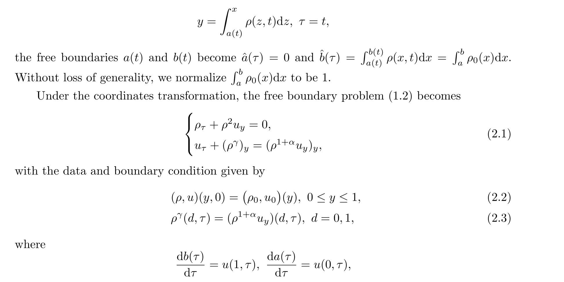
andb(0)=b,a(0)=afor anyb ＞a.

In this section, we mainly consider the asymptotic behavior of the initial boundary value problem (2.1)-(2.3).In fact, the global existence of a weak solution to (2.1)-(2.3) was proven in [14] by the following lemma:

Lemma 2.1Assume that (ρ0,u0) satisfy (A1)-(A2) andγ ＞1, 0＜α ＜1.Then there exists a unique global weak solution to (2.1)-(2.3).

Next, we establisha prioriestimates for (ρ,u) to (2.1)-(2.3).

Lemma 2.2Under the conditions of Theorem 1.2, we have that

whereCis a positive constant independent ofτ.

ProofMultiplying (2.1)2by u and integrating the resulting equation over (0,1)×(0,τ),and using (2.1)1, we obtain the desired estimate.□

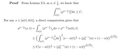
In what follows, we give some useful estimates on the derivative of the density function;this is crucial for obtaining the lower bound of the density.

Lemma 2.5Let the assumptions in Theorem 1.2 be satisfied.Then

Thus, we obtain (2.10) by virtue of (2.4).

as 1＜γ ＜1+α.

The proof of Lemma 2.5 is complete.□

2.1 Decay Rates of the Density Function

At this stage, we will give the decay rates of the density function.To this end, let us introduce that

Thus, the auxiliary functionswandρa(bǔ)re satisfied with

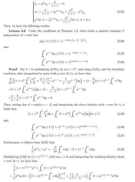
In the next Lemma, with the help of Lemmas 2.3-2.5, we give the time-weighted lower bound of the density function by virtue of the method from [14].

Lemma 2.9Under the conditions of Theorem 1.2, for any 0＜η ?1, there exists a positive constantC(η) independent ofτsuch that

We complete the proof of Lemma 2.9 by combining(2.38)and(2.40)for some large enoughn ∈N+.□

Next, we turn our attention to the optimal decay of the density function.For this, a sufficient condition on the time-weighted lower bound of the density is given.

Proposition 2.10Under the conditions of Theorem 1.2, forγ ＞1+2α, if there exists a uniform positive constantc0such that

ProofWe give the proof in three steps.

Step 1The goal of this step is to obtain the optimal time-weighted upper bound of the density.In fact, we only need to focus on the case 1+2α ＜γ ＜2+α, due to Remark 2.7.

Multiplying(2.25)2byw(1+τ)k,withk ＞0,and using(2.25)1and the boundary condition,after integration by parts withyover (0,1), we have that

Similarly, settingk=k′+∈in (2.44) with any small∈＞0, fork′＜min{2,γ-1},k′≤1-β0(1-α),

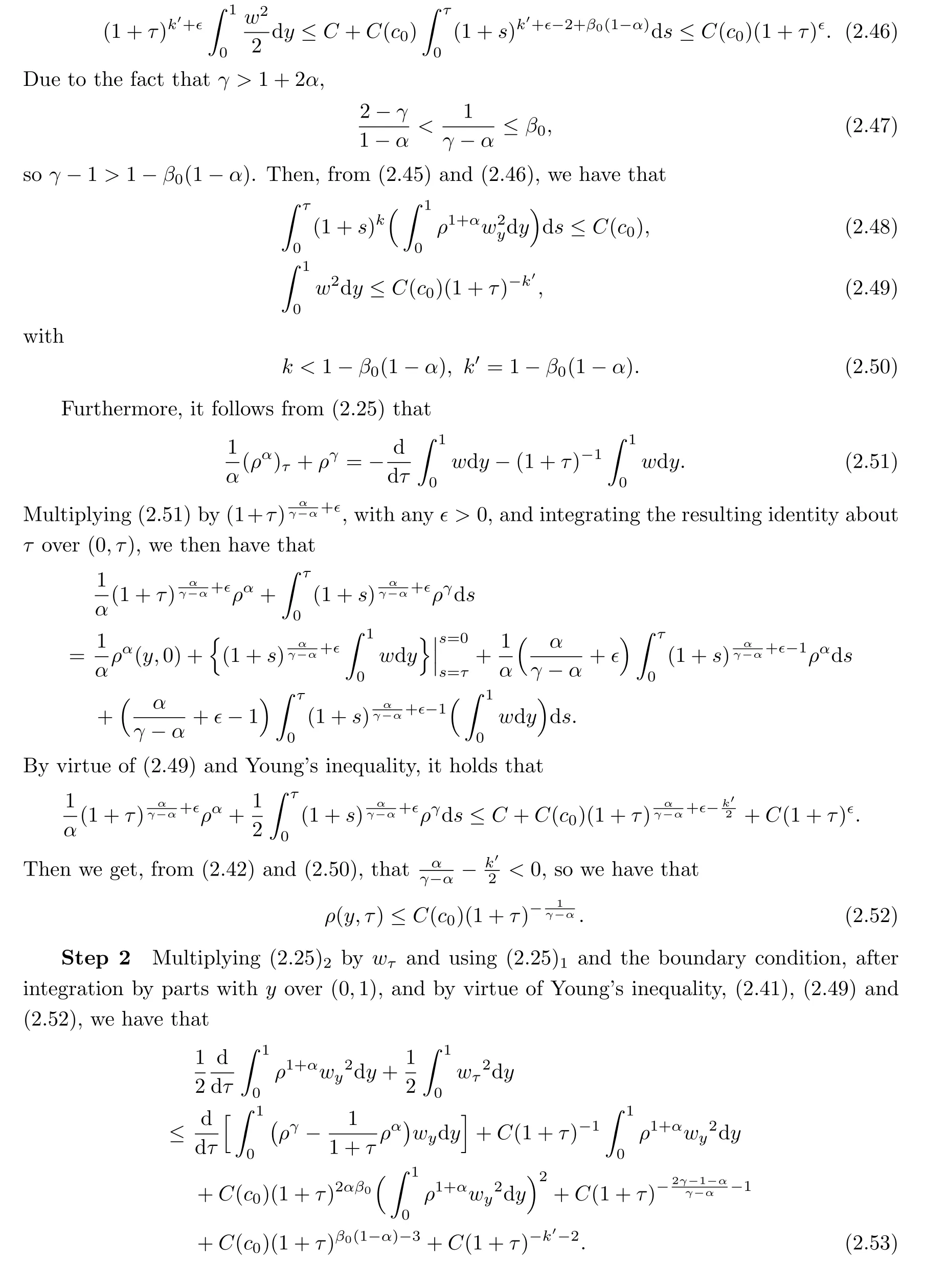
Multiplying (2.53) by (1+τ)land integrating the resulting identity withτover (0,τ), we then have that

This, together with (2.52), proves Proposition 2.10.□

From now until the end of this section we address the Eulerian coordinates, for the convenience of calculation.

2.2 Expanding Rate of the Free Boundary

Lemma 2.11Under the conditions of Theorem 1.2, there exists a positive constantCindependent oftsuch that

2.3 Interface Behavior of the Density Function

The next two Lemmas show the density behavior near the interface.

The proof of (2.77) is similar to that of (2.76).□

Similarly, one can obtain (2.80), due to (2.34).□

Now we are ready to prove Theorem 1.2.

Proof of Theorem 1.2By virtue of thea prioriestimates established in this section and the standard argument used in [14], we can construct the weak solution to the free boundary problem (1.2).Then, by combining Lemmas 2.6 and 2.9, we obtain Theorem 1.2 (i).Theorem 1.2 (ii) is a direct consequence of Lemma 2.11.□

3 Smoothness of the Solution

In this section, we will study the smoothness of the solution constructed in Section 2, and prove Theorem 1.6.

First, we get the following derivative estimates of the velocity function:

Lemma 3.1Under the conditions of Theorem 1.2 andu0yy ∈L2([0,1]), for 0≤τ ≤T,there exists a positive constantC(T) such that

The proof of Lemma 3.1 is complete.□

Next, we have the followingL2-estimate ofρyy(this is crucial for the improvement of regularity of the solution):

Lemma 3.2Under the conditions of Lemma 3.1, ifρ0yy ∈L2([0,1]), then

Thus, we arrive at

This, together with Gr¨onwall’s inequality, leads to the desired estimates.□

Now, we are ready to prove Theorem 1.6.

Proof of Theorem 1.6First, transforming the results in Lemmas 3.1-3.2 back into Eulerian coordinates, by (2.10), (2.26) and (2.34) we can obtain (1.7).Then the standard parabolic theory (please refer to [16]) and the regularity of (ρ,u), which we have obtained,imply the H¨older continuities indicated in Theorem 1.6; see also [17].□

4 Exact Self-similar Solutions

In this section, we turn to the proof of Theorem 1.7, regarding the self-similar solutions to the free boundary problem (1.2).

Note that,by virtue of Remark 2.4,we can find some pointy0∈(0,1)such thatu(y0,τ)=0.Transforming this into Eulerian coordinates, we get that

We first give a Corollary of Theorem 1.7 which shows the optimal estimates and interface behavior of the self-similar solution obtained in Theorem 1.7.

Corollary 4.1It can be verified that the solution, with (1.8)-(1.10) in Theorem 1.7,satisfies the following properties:

(1) the large time behavior of the density and the velocity on the free boundary are

Now we begin by proving Theorem 1.7.In order to choose a suitable function of (ρ,u),we give a self-similar solution to the continuity equation (1.2)1(this was, in fact, obtained in[30, 32] and [8]).

Lemma 4.2For any twoC1functions,f(z) anda(t)/=0, define that

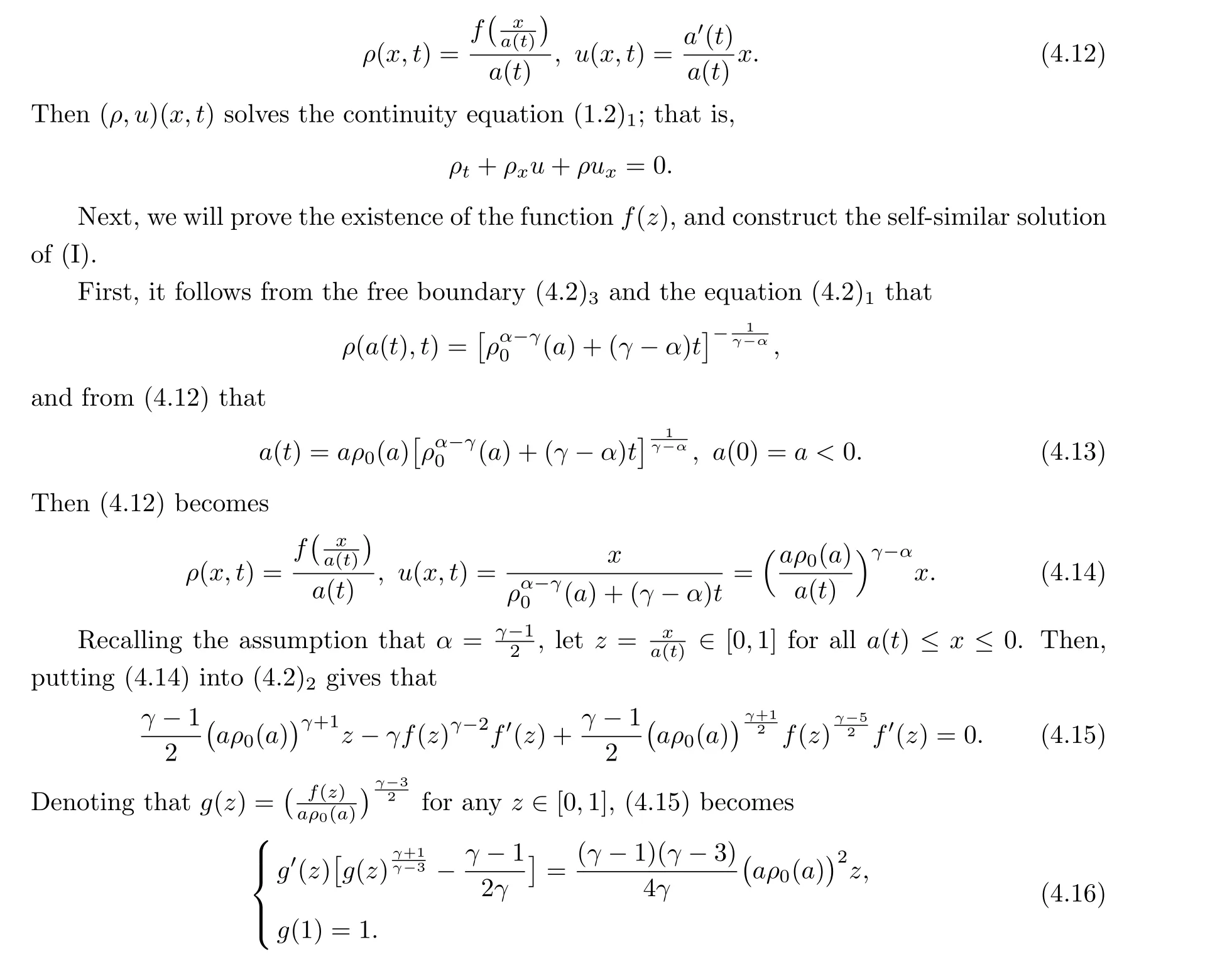
In what follows, we prove that the equation (4.16) can be solved on [0,1].To this end, we start witha prioriestimates and the uniqueness.

Lemma 4.3For any 1＜γ ＜3, letg(z) be a solution to the system (4.16) inC([0,1])∩C1((0,1]).Then

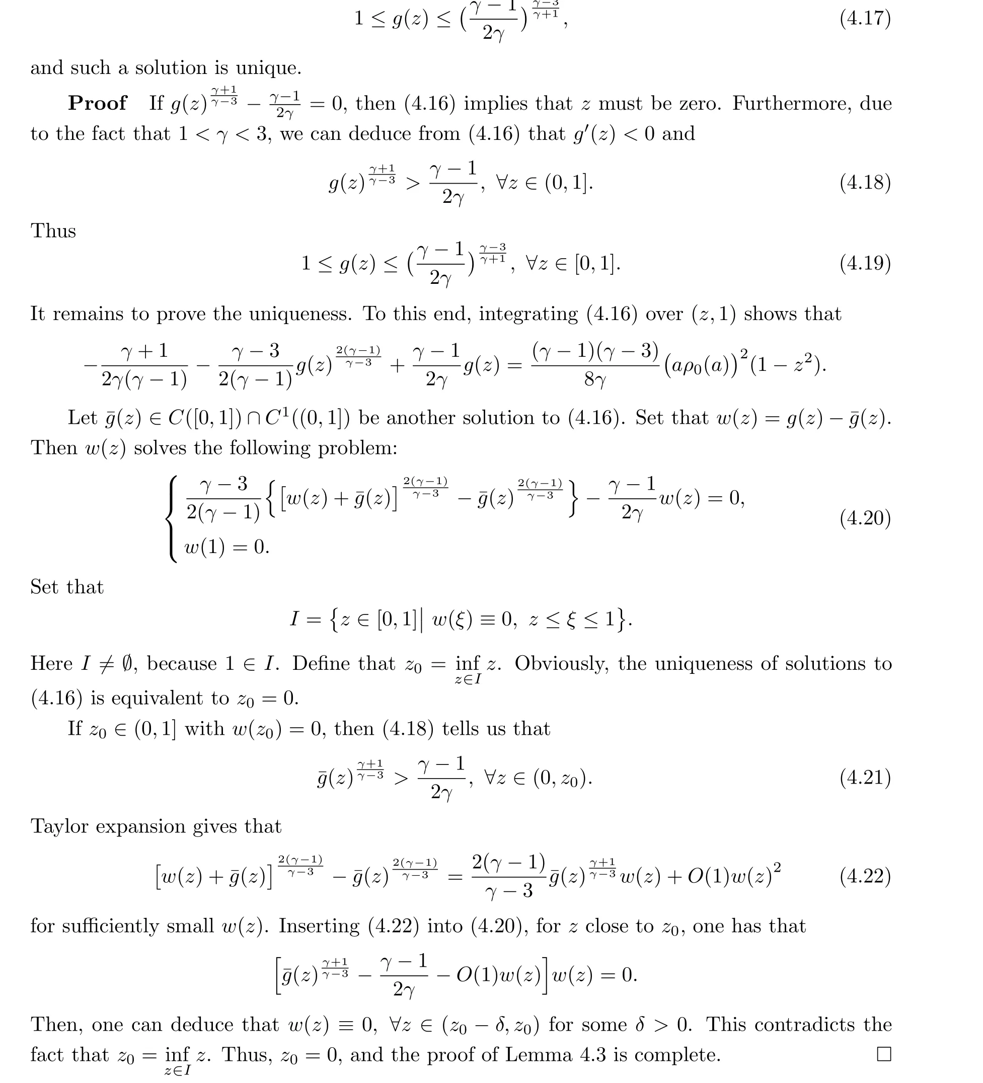
Now, we are ready to give the existence result of system (4.16).

Lemma 4.4For any 1＜γ ＜3, there is a positive functiong(z)∈C([0,1])∩C1((0,1])satisfying (4.16).

Proof We can rewrite (4.16) as follows:

This completes the proof of Lemma 4.5.□

Finally, combining Lemmas 4.2-4.5, we obtain the global existence off(z)∈C1([0,1]) for equation (4.15).Similarly, we can follow the same process for system (II) withf(z) replaced by another function,h(z).Therefore, we now obtain the solutions of (I) and (II):

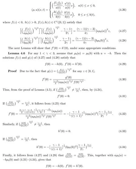
This proves Lemma 4.6.□

With the help of Lemma 4.6, we can now combine (4.26) into a unified solution of the free boundary problem (1.2) for anya(t)≤x ≤b(t), and further complete the proof of Theorem 1.7.

Proof of Theorem 1.7Under the conclusions of Lemmas 4.2-4.6, by (4.13), (4.27),(4.28) and (4.29), we have that

Conflict of InterestThe authors declare no conflict of interest.