Reconstruction of poloidal magnetic field profiles in field-reversed configurations with machine learning in laser-driven ion-beam trace probe

Xutao XU (徐栩濤) ,Tianchao XU (徐田超),* ,Chijie XIAO (肖池階),* ,Zuyu ZHANG (張祖煜) ,Renchuan HE (何任川) ,Ruixin YUAN (袁瑞鑫) and Ping XU (許平)

1 State Key Laboratory of Nuclear Physics and Technology,School of Physics,Peking University,Beijing 100871,People’s Republic of China

2 School of Physics,Xihua University,Chengdu 610039,People’s Republic of China

Abstract The diagnostic of poloidal magnetic field (Bp) in field-reversed configuration (FRC),promising for achieving efficient plasma confinement due to its high β,is a huge challenge because Bp is small and reverses around the core region.The laser-driven ion-beam trace probe (LITP) has been proven to diagnose the Bp profile in FRCs recently,whereas the existing iterative reconstruction approach cannot handle the measurement errors well.In this work,the machine learning approach,a fast-growing and powerful technology in automation and control,is applied to Bp reconstruction in FRCs based on LITP principles and it has a better performance than the previous approach.The machine learning approach achieves a more accurate reconstruction of Bp profile when 20% detector errors are considered,15% Bp fluctuation is introduced and the size of the detector is remarkably reduced.Therefore,machine learning could be a powerful support for LITP diagnosis of the magnetic field in magnetic confinement fusion devices.

Keywords: FRC,LITP,poloidal magnetic field diagnostics,machine learning

1.Introduction

The field-reversed configuration (FRC) is a compact torus and a promising magnetic confinement fusion (MCF)concept due to its high β [1,2].It is a fascinating fusion concept that falls in between magnetic fusion and inertial fusion.There is great anticipation for the actualization of nuclear fusion through this concept.The poloidal magnetic fieldBpis critical for the study of plasma equilibrium,confinement and transport.However,theBpin FRCs is small and reversed around the core region,causing great difficulties in terms of traditionalBpdiagnostic approaches.The laser-driven ion-beam trace probe (LITP) has been proposed to diagnose theBpand the radial electric field (Er)profiles in tokamaks [3-6],and the feasibility of using LITP diagnostics to reconstruct the internal magnetic field in FRCs has been verified recently [7].An iterative approach with a dissipative term has been developed.When the random noise is relatively small,reconstruction results provided by this approach are consistent with the preset.However,the reconstructed profile deforms seriously and the relative reconstruction errors are almost 25% when 10%random noise is added [7].Considering the noise caused by practical conditions like mechanical vibration,the iterative approach would not meet the requirement of experimentalLITP diagnosis.

As a fast-growing and powerful technology in the field of automation and control,the machine learning approach has been already used successfully to solve several challenging issues in the MCF domain,including the prediction of disruptions in fusion devices,tokamak magnetic control,reconstruction of the last closed-flux surface on tokamaks,reconstruction of the plasma boundary on tokamaks and so on [8-11].In order to make up for the deficiency of the iterative reconstruction approach mentioned above,a machinelearning algorithm is used in the LITP to reconstruct theBpprofile by generating a non-linear mapping relation between the toroidal displacement of ions and theBpprofiles.In this work,a machine-learned LITP approach is developed and its performance in terms of reconstructingBpprofiles in FRCs is numerically verified.A neural network is trained with datasets generated by an orbit simulation program.The relative error of the reconstructedBpis below 20% in most areas with up to 20% random noise added on the displacement of ions.When theBpfluctuation is under 15%,the reconstruction results of the machine-learning approach are close to the preset and only one 35 × 5 cm2detector is needed,reducing the port requirements.Thus,the application of the machinelearning algorithm in LITP can effectively improve its performance,making it more feasible to experimentally diagnose magnetic field in FRC devices.

In this article,the principle of LITP diagnosis in FRCs is introduced in section 2.The training architecture is illustrated in section 3.The reconstruction results using both an iterative approach and a machine-learned approach are presented and compared in section 4.Section 5 includes the discussions and conclusions.

2.Principles of LITP diagnosis in FRCs

The principle of LITPBpdiagnosis for FRCs has been derived in the previous work [7].The reconstruction of theBpprofile in the FRC mid-plane is considered first of all.The magnetic configuration,as shown in figure 1,can be assumed to be symmetric in the toroidal direction and symmetric about the mid-plane.Therefore,the radial magnetic field (Br) can be assumed to be zero.AsBtis much smaller thanBpin FRCs,it is reasonable to assumeBt=0 andB=Bpez,andEis set as zero because the displacement caused byE～103V/m is approximately several millimeters for protons [7].

When an ion of a laser-driven ion beam (LIB) passes through the FRC device chamber perpendicular to the poloidal magnetic field,there will be a toroidal displacement Φtdue to the Lorentz force ofBp.Since the LIB has large energy spread,ions with different energies will spread in the toroidal direction.According to the previous theoretical derivation,the toroidal displacement can be expressed as Φt-2α0is the toroidal incidence exit angle.According to this principle,the profiles ofBpcan be reconstructed when enough ion traces are provided.An iterative approach was developed to reconstruct theBpprofile.Firstly,an initialBpprofile is provided to calculate the first set of ion orbits.With the information of toroidal displacement Φt,a newBpprofile will be solved.These steps are repeated and iteration stops when a convergent condition is satisfied.

In the previous work,the iterative method behaved poorly with above 10% noise.In order to improve the reconstruction performance,the machine-learning algorithm is developed to replace the iterative method in LITP.

3.Training architecture for LITP diagnosis

The training architecture is depicted in figure 2,which is a flexible approach for LITP reconstruction in different magnetic configuration devices.The approach has three main phases.Firstly,given a specific magnetic field,an orbit simulation program calculates the displacement of injected ions to generate a set of data.This process is repeated with different magnetic fields each time until enough datasets are obtained.Secondly,a neural network is trained using the displacement data series as input and the corresponding magnetic field as target.Then,the well-trained neural network model,which has learned to find optimal mapping from a displacement data series to the magnetic field,should be able to reconstruct the magnetic field using the measured displacement of ions.

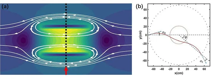
Figure 1.(a) Schematic diagram of the FRC magnetic field.The black dashed line indicates the mid-plane.(b) Schematic trace projection diagram of one ion in the mid-plane.

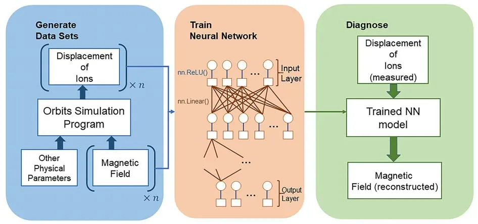
Figure 2.The training architecture.Generate data sets: the orbit simulation program calculates the displacement of ions on the basis of a preset magnetic field and other physical parameters.Train neural network: a neural network algorithm runs with the displacement of ions as input and the corresponding magnetic field as target.Diagnose: a trained neural network (NN) model is able to reconstruct the magnetic field with the measured displacement of ions.

In this work,our orbit simulation program calculatesΦtof 500 ions for each presetBpprofile,which is discretized into 40 concentric ring pixels in the radial direction.The preset magnetic field profile is approximated using a hyperbolic tangent function [12,13],which is expressed as

whereB0,kandR0are the variable parameters,referring to the edge poloidal magnetic field,the width of the variable region ofBpand the radius of theBpinversion point,respectively,andris the radius position in the mid-plane.The model of the magnetic field profile in FRCs,described by equation (1),is the simplest rigid rotor FRC profile model and the most widely used and adopted model in the experiment [14,15].In order to compare the reconstruction performance of these two approaches,the same model described by equation (1) is used.

To generate large number of datasets for training,B0,kandR0are taken as uniform random numbers within[400,3000](G),[0.2,3.0] and [0.2,0.5](m),respectively.The range selection of these parameters is discussed in previous work [7].We use 10000 sets of data to train a simple multi-layer perceptron neural network.The input layer has 500 nodes,corresponding to the toroidal displacement of 500 ions.The output layer,of course,has 40 nodes according to the discretization of theBpprofile.Each layer is a linear layer that applies a linear transformation to the incoming data:y=xAT+b.Apart from the nodes in the input layer,each node uses a rectified linear unit as its activation function.The optimization process of adjusting model parameters is performed using standard backpropagation methods with mean square error cost function.

4.Reconstruction of Bp in FRCs through machine learning

4.1.Optimization of orbits

The energy of the protons ranges from 100 keV to 600 keV,which requires 4 TW femtosecond lasers [7].The presetBpprofile used in the discussion below is given by equation (1)withB0=1000 G,k=1 andR0=21 cm.First,the displacement data collected by two 35 × 5 cm2detectors is used to reconstruct the presetBpprofile,as shown in figure 3(a).The reconstruction results using the previous iterative LITP approach and the machine-learned LITP approach are compared in figure 3(b) .The reconstruction value by machine learning,marked in blue,is quite close to the preset value.Compared with the iterative approach,the relative error of the machine-learned approach is smaller in the edge area but bigger around the reverse location ofBp.Overall,the reconstruction results of both two approaches meet the expectation for LITP.

In order to improve the applicability of LITP poloidal magnetic field diagnostics in FRCs,the size of the detector needs to be smaller to reduce the requirement for a viewing port.Thus,we tested these two approaches with only one 35×5 cm2detector.The position of the detector and a fraction of the detected ion traces are shown in figure 4(a).

The reconstruction results using two approaches are shown in figure 4(b).The reconstruction value by the iterative approach (marked in red) deforms seriously when only one detector is used,which means the performance of the iterative approach declines sharply with the reduction of ion traces.The reconstruction results from the machine-learned LITP approach (marked in blue) are similar to the results from the two detectors,revealing that the machine-learned approach could maintain an accurate reconstruction performance.

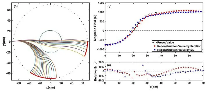
Figure 3.(a) A fraction of the detected ion traces.The position of the detector is represented by the circular arc line.(b) The reconstruction results using iterative and machine-learned LITP approaches and (c) the distribution of each approach’s relative error.

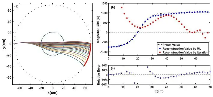
Figure 4.(a) A fraction of the detected ion traces (using one detector).The position of the detector is represented by the circular arc line.(b) The reconstruction results using iterative and machine-learned LITP approaches (using one detector) and (c) the distribution of the relative error of the machine-learned LITP approach.

4.2.The effect of measurement errors

In order to inspect the effect of measurement errors for the machine-learned approach,random noise is added to the toroidal displacement of ions on the detector.Figure 5 shows the reconstruction results and the relative errors.When 10%noise is added,most of the relative errors with the iterative approach,shown in figure 5(c),are above 25%.By using the machine-learned LITP approach,the relative errors shown in figure 5(a) are mostly under 10%,except for the area around the reversed location.

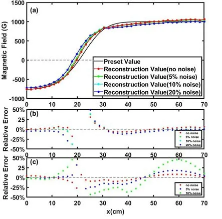
Figure 5.(a) The reconstruction result using the machine-learning approach with one detector is represented by the red line.When 5%,10% and 20% random noises are added in the toroidal displacement,the reconstruction results are marked in green,bluegreen and blue respectively.(b) The distribution of corresponding relative errors using machine-learning approach.(c) Red dots are the relative errors using the iterative approach with two detectors.When 5% and 10% random noises are added in the toroidal displacement,the relative errors of reconstruction are marked in blue and green.respectively.

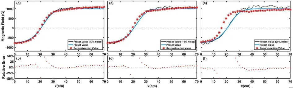
Figure 6.The reconstruction results and the relative errors under different levels of random noise added to the magnetic field.(a) and (b) 10%random noise is added to the preset magnetic field profile.(c) and (d) 15% random noise is added to the preset magnetic field profile.(e) and (f) 20% random noise is added to the preset magnetic field profile.The reconstruction result starts to deform.

4.3.The effect of poloidal magnetic field fluctuation

The noise in real experimental scenarios would come not only from detector measurement errors,but also the poloidal magnetic field fluctuation.In order to find out the effect of magnetic field fluctuation and assess the robustness of the machine-learned LITP approach,random relative noise is added to the presetBpprofiles.We have added 10%,15%and 20% random noises to the preset poloidal magnetic field,respectively.The reconstruction results and the relative errors are shown in figure 6.The relative reconstruction errors are below 10% in most regions when 10% and 15%noise is added.In the region around 20 cm,the relative error is up to 50% because the magnetic field is relatively small.When 20% noise is added,the reconstruction results are poor in the region of 10-30 cm and the inversion point moves about 5 cm.Therefore,the machine-learning approach can tolerate 15% poloidal magnetic field fluctuation.

The reconstruction results demonstrate that,compared to the iterative LITP approach,the machine-learned LITP approach has higher reconstructing accuracy and works well with fewer ion traces,up to 20% random noise of toroidal displacement and 15% magnetic field fluctuation.The results prove that the application of a machine-learning model improves the performance of LITP diagnostics,making it more feasible for FRC magnetic field measurements in more restricted experimental conditions.

5.Conclusion

The application of a machine-learning model to LITP diagnostics of FRC magnetic fields is verified numerically.The reconstruction performance of the machine-learned LITP approach is tested under the conditions of smaller detectors,up to 20% detector errors and 15% magnetic field fluctuation.By comparing with the previous iterative approach,the reconstruction results manifest that the application of the machine-learning model improves the performance of LITP diagnostics and is robust,showing a promising future of LITP diagnosing theBpof FRCs in experiments.

The FRC profile model used in this study has the disadvantage of stiffness.A more generalized two-parameter modified rigid rotor (MRR) model has been proposed,which has solved the problem of profile stiffness and could effectively describe the magnetic profile when the plasma density near the wall is non-negligible [14].LITP diagnosis using the MRR model will be considered in our future research,and the two-dimensionalBpdiagnostic in FRCs and the diagnostic forErwill be explored with the application of more complex machine-learning algorithms in LITP.

Acknowledgments

This work was supported by the National MCF Energy R&D Program of China (No.2018YFE0303100) and National Natural Science Foundation of China (No.11975038).