Growth curve mixture models

Benjamin E. LEIBY

· Biostatistics in psychiatry (12) ·

Growth curve mixture models

Benjamin E. LEIBY

Psychiatric studies often collect longitudinal data to characterize the natural history of disease in a cohort or to evaluate the effect of behavioral or pharmaceutical interventions. For example, in a recent partially randomized study comparing escitalopram and nortriptyline in the treatment of depression, several depression scales were measured weekly over the 3-month course of treatment.[1]While the primary outcome measure of such studies may be a binary indicator of improvement at the end of treatment, analysis of the full longitudinal profile that makes optimal use of all available data to model rates of change over time may be more informative. For example, in the escitalopram/nortiptyline study, analysis of dichotomous outcomes adjusted for time participating in the study showed no difference between drugs, while analysis of the longitudinal profiles did indicate different patterns of improvement in the two groups over time.[2]

1. Mixed effects models

Mixed effects models[3]have become the standard for analysis of data from longitudinal studies that assess the behavior of a single continuous outcome over time. In general, mixed effects models model the average trend in a single variable over time while allowing for subjectspecific deviations from this trend. As an example, consider a 2-arm clinical trial (active drug vs. placebo) where treatment for depression reduces depressive symptoms as measured by the Hamilton depression rating scale (HAMD). Each subject has a certain level of symptoms when beginning treatment (the intercept), and a rate of change in depressive symptoms over time (the slope). If a treatment is effective, the rate of decline for subjects randomized to active treatment will be different from (greater than) that of those randomized to placebo. The focus of analysis is the comparison of the average slope for those on active treatment to the average slope for those on placebo. Mixed effects models formalize this idea by specifying a subject-level model with subject-level parameters which are then related to population-level parameters. In our example, we might specify the subject-level model as

whereyijis the HAMD score at timej, β0iand β1iare the intercept and slope for subjecti, andeijis normally (i.e., bell-shaped) distributed random noise. Thus, we assume that each subject’s HAMD scores at the different followup times have a linear relationship (i.e., are on a straight line) over time. We relate each subject’s intercept and slope to a population average intercept and slope:

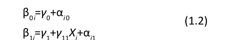
whereXi=1 for subjects assigned to treatment,Xi=0 for subjects assigned to placebo,γ0is the average intercept,γ1is the average slope for placebo patients,γ1+γ11is the average slope for treated patients, and αi0and αi1are normally distributed random variables that allow each subject’s intercept and slope to differ from the average. The effectiveness of the treatment is determined by testing the null hypothesis thatγ11=0, in which case the rate of decline is the same in placebo and treated patients.

The mixed effects model assumes that subjects’intercepts and slopes are relatively homogeneous with variation centered around one central line. However, there are cases where this may not be a reasonable assumption. In a time when ‘personalized medicine’ is the goal, it is becoming increasingly clear that many, if not most, diseases are not homogeneous. Different subpopulations may have distinct natural histories and may respond to treatment in different ways. Thus, models that consider the whole population and average across multiple subtypes may miss important differences in the effects of treatment. Without a prior knowledge of these subtypes it can be difficult to account for them. Models incorporating latent class are one way of investigating this type of unobserved population stratification or clustering. Originally developed for cross-sectional data, classical latent class models are a type of finite mixture model where the focus is to identify a finite number of subgroups based on multiple outcomes.[4,5]

2. Growth curve mixture models

In the past two decades, many researchers have focused on extending latent class models to consider grouping subjects based on trajectories or growth curves rather than only on cross-sectional data. Growth curve mixture models (GCMMs[6]) are a type of latent variable model that extend the latent class model to the longitudinal setting where subjects are grouped based on the observed longitudinal trend over time. (For a brief review of latent variable modeling, see Cai[7]). This approach assumes that each subject belongs to a certain unobserved group (the latent class) and subjects in that class have a particular mean trajectory. In essence, each latent class has its own mixed effects model. IfCi=kindicates that subjectibelongs to classk, then we have

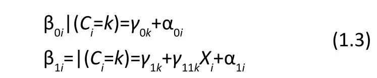
where β0i|(Ci=k) and β1i=|(Ci=k) denote the intercept and slope for subjectigiven that the latent class membership for subjectiis groupk. Estimates are obtained for growth curve parameters (e.g., intercepts, slopes, etc.) for each latent class.

It is important to note that although the model assumes that subjects belong to one of the classes, the class membership is unknown and the results of the analysis can only assign subjects to a given class with a certain probability. To do this, after the model is estimated, each subject’s observed data are compared with the resulting class-specific curves. The closer the subject’s data resemble the class-specific curve, the higher the probability of belonging to that class. Based on this probability, subjects can be assigned to their most likely class and factors associated with class membership can be investigated.

GCMMs can be used in many ways. At their most basic, they can be used to identify subgroups whose observed trajectories look similar to each other but different from the other subgroups. For example, investigators in the aforementioned drug trial categorized subjects based on their pattern of depressive symptoms during a 12-week treatment period[2]and identified two classes –gradual improvers and rapid improvers. Once patterns are discovered, the association of other factors with these patterns may provide insight into risk factors for an outcome or predictors of improvement. In the drug trial, one of the treatments was more prevalent among the rapid improvers than the other.

In randomized trials, the type of interventions administered can also be taken into consideration when creating the classes. When adding this factor to the longitudinal model, the identified classes may differ not only with respect to the shape of the average trajectory, but also with respect to the magnitude of the treatment effect. In conditions that are very heterogeneous, the results of this analysis may be able to identify the distinct subgroups in which the intervention of interest is effective.[8]

Originally developed for single continuous outcomes, extensions to the GCMM methodology allow for the analysis of categorical outcomes[9]and of multiple outcomes.[10,11]GCMMs can also be used to jointly model longitudinal processes and distal outcomes, and can be an effective way of modeling the relationship between biomarkers and event times.[12]

3. Practical considerations for growth curve mixture modeling

Jung and Wickrama[13]provide a good review of GCMMs and their implementation. GCMMs require specification of the number of latent classes prior to fitting the model. The choice of this number is not easy. Standard likelihood ratio tests for choosing between models cannot be used, but adjustments to the standard test that can help in the decision about the number of latent classes to be used in the model are available in some software packages. Information criteria (e.g., Akaike information criteria, or Bayesian information criteria) can also be used to compare models to choose the number of classes with the best fit. GCMM analysis is usually exploratory; the models can become complex fairly quickly, so to avoid spurious results or generating models with more parameters than the data can support, clinical and scientific knowledge should guide the modeling.

Software for fitting GCMMs is fairly specialized and generally unavailable in standard statistical packages. Recently, the R-package LCMM has been developed to fit some types of GCMMs including joint models for longitudinal and time-to-event data (http://cran.rproject.org/web/packages/lcmm/). The most widely used software is Mplus[14]which provides modeling capabilities for an extensive array of GCMMs in addition to other latent variable methods such as factor analysis and structural equation modeling.

A special case of GCMMs is latent class growth analysis (LCGA)[15,16]which does not allow for departure from the average trajectory within each latent class (by setting α0iand α1iequal to zero in equation 1.3). Thus, in contrast to mixed effects models where each subject’s intercept and slope are drawn from a normal distribution or GCMMs where they are drawn from a mixture of normal distributions, LCGAs allow only for a limited set of discrete options (one possibility for each class). LCGA can be implemented using the specialized SAS procedure Proc Traj.[17]

4. An example

The following simulated example demonstrates the uses of GCMMs in the analysis of longitudinal data from a clinical trial. The simulated data set contains weekly HAMD scores for 100 patients randomized to placebo or active treatment for 10 weeks. A standard analysis of this data would apply the mixed effects model outlined above. The subject-specific trajectories of HAMD scores and the estimated population curves for placebo and treated patients resulting from this analysis are given in Figure 1. On average, placebo patients’HAMD scores decreased by 0.33 points per week, while the active treatment groups’ scores declined by 0.54 points per week. The difference in rates of decline was not statistically significant (p=0.053). While strict interpretation of the results would conclude that the treatment was not effective, a visual examination of the plots shows a substantial number of patients in the active treatment arm that had much greater decline than average. This suggests that there may be a subset of patients for whom the treatment was effective.

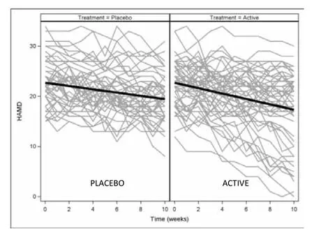
Figure 1. Simulated observed HAMD scores by subject and model-estimated curves from the mixed effects model

A GCMM analysis that allows for differing effects of treatment within each class was fit using Mplus. A model with two classes fit best, and subjects were assigned to their most likely class with 67 subjects assigned to class 1 and 33 assigned to class 2. Results are displayed graphically in Figure 2. Class 1 was categorized by similar minimal rates of decline in treated and placebo subjects (slopes of -0.105 and -0.087, respectively, p=0.53). In Class 2, both treated and placebo subjects declined more than in Class 1, but treated subjects improved about two-fold more quickly than placebo subjects (slopes of -1.545 and -0.754, respectively, p＜0.001). Further investigation would be warranted to identify baseline characteristics that differed between the two latent classes; these characteristics would help identify the type of patients for whom the drug would be beneficial.

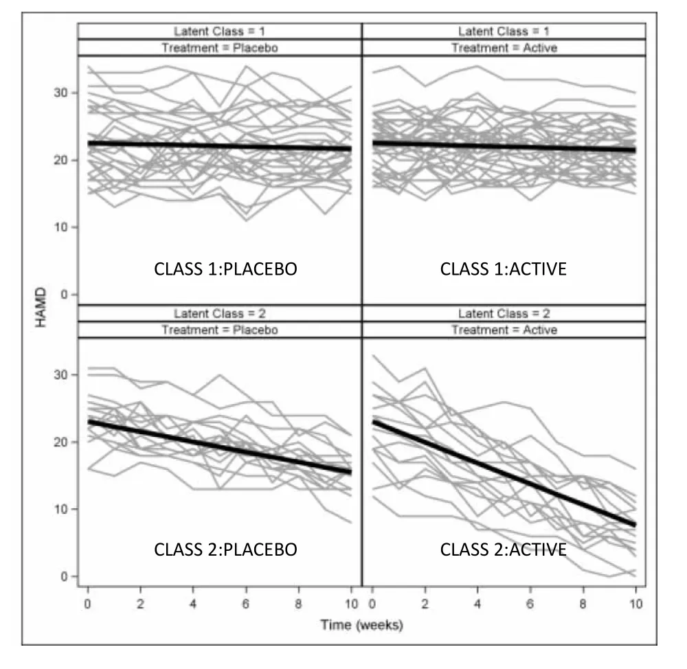
Figure 2. Results of a GCMM applied to the same data. Treated subjects in class 2 have greater decline than placebo subjects

An alternative GCMM analysis could ignore treatment in forming the classes based on the HAMD trajectories. Again, a 2-class model fits best, as depicted in Figure 3. In this analysis, the model identifies a small class of subjects (n=16) whose HAMD scores decline by 1.49 points per week. A cross-tabulation with treatment assignment reveals a significant association between class and treatment assignment (p＜0.001) with all 16 improvers being assigned to active treatment. Again, post-hoc comparisons of subjects who did and did not improve with treatment would help identify the demographic and clinical characteristics of patients who are most likely to improve.

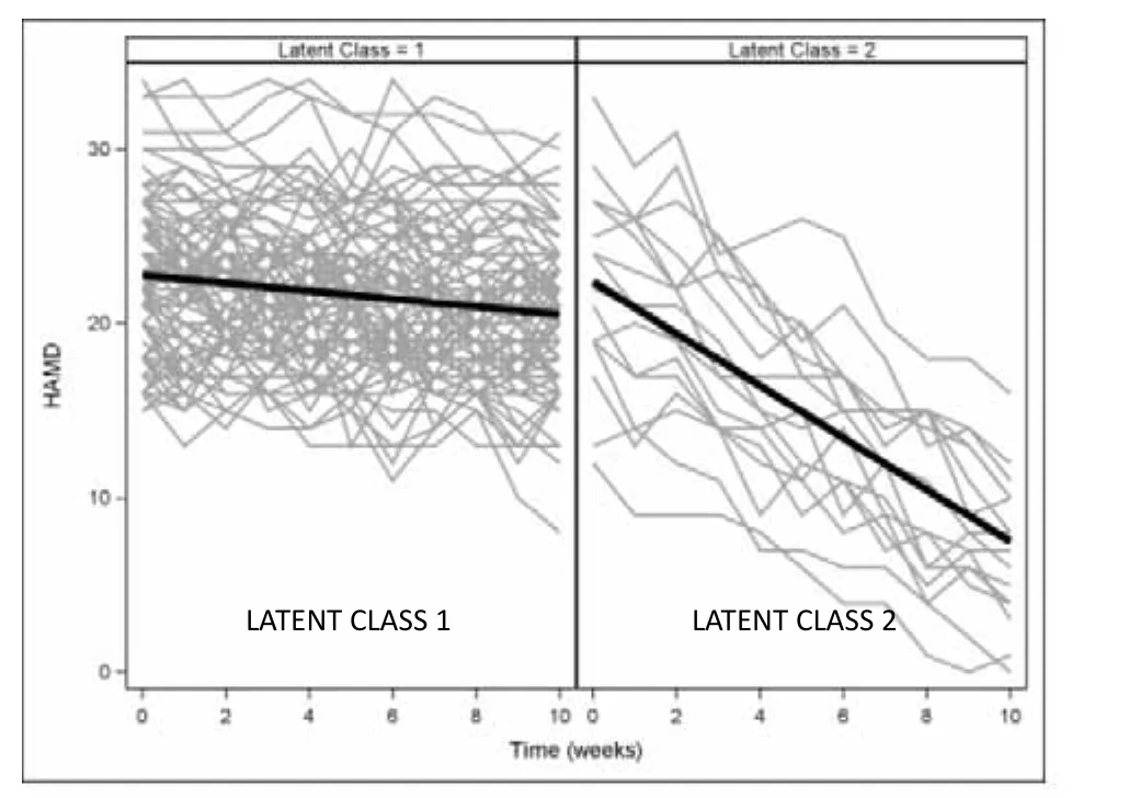
Figure 3. Results of a GCMM ignoring treatment assignment

5. Conclusion

Growth curve mixture modeling can be a useful analysis tool when it is desirable to identify subgroups of patients who differ with respect to the trajectory of a longitudinal measurement. GCMMs extend commonly used mixed effects methods to allow for multiple classes, each with its own mixed effects model. These models are useful in observational and experimental studies, and they provide a method for identifying subgroups of patients who respond differently to interventions in randomized trials.

1. Uher R, Maier W, Hauser J, Marusic A, Schmael C, Mors O, et al. Differential efficacy of escitalopram and nortriptyline on dimensional measures of depression.Br J Psychiatry2009; 194(3): 252-259.

2. Uher R, Muthen B, Souery D, Mors O, Jaracz J, Placentino A, et al. Trajectories of change in depression severity during treatment with antidepressants.Psychol Med2010; 40(8): 1367-1377.

3. Laird N, Ware J. Random-effects models for longitudinal data.Biometrics1982; 38: 963-974.

4. Clogg CC. Latent class models. In: Arminger G, Clogg CC, Sobel ME, eds.Handbook of Statistical Modeling for the Social and Behavioral Sciences. New York: Plenum Publishing Corporation, 1995.

5. Garrett ES, Zeger SL. Latent class model diagnosis.Biometrics2000; 56: 1055-1067.

6. Muthén B, Asparouhov T. Growth mixture modeling: Analysis with non-Gaussian random effects. In: Fitzmaurice G, Davidian M, Verbeke G, Molenberghs G, eds.Longitudinal Data Analysis. Boca Raton: Chapman Hall/CRC Press, 2008:143-165.

7. Cai L. Latent variable modeling.Shanghai Arch Psychiatry2012; 24(2): 118-120.

8. Muthén B, Brown CH, Masyn K, Jo B, Khoo ST, Yang CC, et al. General growth mixture modeling for randomized preventive interventions.Biostatistics2002; 3(4): 459-475.

9. Muthén B, Shedden K. Finite mixture modeling with mixture outcomes using the EM algorithm.Biometrics1999; 55: 463-469.

10. Elliott MR, Gallo JJ, Ten Have TR, Bogner HR, Katz IR. Using a Bayesian latent growth curve model to identify trajectories of positive affect and negative events following myocardial infarction.Biostatistics2005; 6:119-143.

11. Leiby BE, Sammel MD, Ten Have TR, Lynch KG. Identification of multivariate responders/non-responders using Bayesian growth curve latent class models.J R Stat Soc Ser C Appl Stat2009; 58: 505-524.

12. Lin H, Turnbull B, McCulloch C, Slate E. Latent class models for joint analysis of longitudinal biomarker and event process data.J Am Stat Assoc2002; 97: 53-65.

13. Jung T, Wickrama K. An introduction to latent class growth analysis and growth mixture modeling.Soc Personal Psychol Compass2008; 2: 302-317.

14. Muthén LK, Muthén BO.Mplus User's Guide (Seventh Edition). Los Angeles, CA: Muthén and Muthén, 1998-2012.

15. Nagin DS, Land KC. Age, Criminal careers, and population heterogeneity specification and estimation of a nonparametric mixed poisson model.Criminology1993; 31: 327-362.

16. Roeder K, Lynch KG, Nagin DS. Modeling uncertainty in latent class membership: A case study in criminology.J Am Stat Assoc1999; 94: 766-776.

17. Jones BL, Nagin DS. Advances in group-based trajectory modeling and an SAS procedure for estimating them.Sociol Method Res2007; 35: 542-571.

Benjamin Leiby is assistant professor in the Division of Biostatistics of Thomas Jefferson University, Philadelphia, Pennsylvania, USA and an associate member of the Kimmel Cancer Center. He collaborates with researchers in a diverse set of fields including cancer, psychiatry, ophthalmology, and rehabilitative medicine. His methodological interests are in the area of latent variable and latent class models with special focus on applications in psychiatry and cancer.

10.3969/j.issn.1002-0829.2012.06.009

Division of Biostatistics, Thomas Jefferson University, Philadelphia, Pennsylvania, USA

*Correspondence: benjamin.leiby@jefferson.edu