Solution of Algebraic Lyapunov Equation on Positive-Definite Hermitian Matrices by Using Extended Hamiltonian Algorithm

Muhammad Shoaib Arif,Mairaj Bibiand Adnan Jhangir

1 Introduction

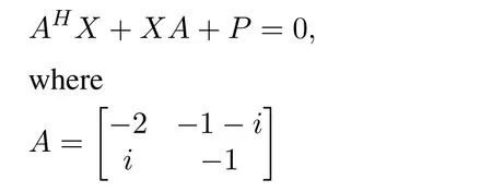
It is well known that many engineering and mathematical problems,say,signal processing,robot control and computer image processing[Cafaro(2008);Cohn and Parrish(1991);Barbaresco(2009);Brown and Harris(1994)],can be reduced as obtaining the numerical solution of the following algebraic Lyapunov equation

wherePis a positive-definite Hermitian matrix,Hdenotes the conjugate transpose of a Hermitian matrix.

The solution of the algebraic Lyapunov equation is gaining more and more attention in the field of computational mathematics[Datta(2004);Golub,Nash and Vanloan(1979)].Several algorithms are used to get the approximate solution of the above-mentioned equation.For instance,Ran et al.[Ran and Reurings(2004)]put forward the fixed point algorithm,the Cholesky decomposition algorithm was presented by Li et al.[Li and White(2002)],and a preconditioned Krylov method to get the solution of the Lyapunov equation was given by Jbilou[Jbilou(2010)].Vandereycken et al.[Vandereycken and Vandewalle(2010)]provided a Riemannian optimization approach to compute the low-rank solution of the Lyapunov matrix equation.Deng et al.[Deng,Bai and Gao(2006)]designed iterative orthogonal direction methods according to the fundamental idea of the classical conjugate direction method for the standard system of linear equations to obtain the Hermitian solutions of the linear matrix equationsAXB=Cand(AX,XB)=(C,D).Recently,Su et al.[Su and Chen(2010)]proposed a modified conjugate gradient algorithm(MCGA)to solve Lyapunov matrix equations and some other linear matrix equations,which seemed to be the generalized results.The traditional method like modified conjugate gradient algorithm(MCGA)are first order learning algorithms,hence the convergence speed of MCGA is very slow.

Another interesting approach to solve algebraic Lyapunov equation is by considering the set of matrices as a manifold and applying the techniques from differential geometry and information geometry.Recently Arif et al.[Arif,Zhang and Sun(2016)]solved the algebraic Lyapunov equation on matrix manifold by information geometric algorithm.Duan et al.[Duan,Sun and Zhang(2014);Duan,Sun,Peng and Zhao(2013)]solved continuous algebraic Lyapunov equation and discrete Lyapunov equation on the space of positivedefinite symmetric matrices by using natural gradient algorithm.Also,Luo et al.[Luo and Sun(2014)]gives the solution of discrete algebraic Lyapunov equation on the space of positive-definite symmetric matrices by using Extended Hamiltonian algorithm.In both the papers,the authors have considered the set of positive-definite symmetric matrices as a matrix manifold and used the geodesic distance betweenAHX+XAand-Pto find the solution matrixX.

Up to date,however,there has been few investigation on the solution problem of the Lyapunov matrix equation in the view of Riemannian manifolds.Chein[Chein(2014)]gives the numerical solution of ill posed positive linear system he combines the methods from manifold theory and sliding mode control theory and develop an affine nonlinear dynamical system.This system is proven asymptotically stable by using argument from Lyapunov stability theory.

In this article,a new frame work is proposed to calculate the numerical solution of continuous algebraic Lyapunov matrix equation on the space of positive-definite Hermitian matrices by using natural gradient algorithm and Extended Hamiltonian algorithm.Moreover,we present the comparison of the solution obtained by the two algorithms.

Note that this solution is a positive definite Hermitian matrices is a global asymptotically stable linear system and the set of all the positive definite Hermitian matrices can be taken as a manifold.Thus,it is more convenient to investigate the solution problem with the help of these attractive features on the manifold.To address such a need,we focus on a numerical method to solve the Lyapunov matrix equation on the manifold.

The gradient is usually adapted to minimize the cost function by adjusting the parameters of the manifold.However,the convergence speed can be seen to be slow if a small change in the parameters changes largely the cost function.In order to overcome this problem of poor convergence,the work has been done in two different directions.Firstly,Amari et al.[Amari(1998);Amari and Douglas(2000);Amari(1999)]introduced the Natural Gradi-ent Algorithm(NGA)which employed the Fisher information matrix on the Riemannian structure of manifold based on differential geometry.Another approach is based on the inclusion of momentum term in the ordinary gradient method to enhance the convergence speed.This is a second-order learning algorithm that was developed by Fiori et al.[Fiori(2011,2012)],which is called the Extended Hamiltonian Algorithm(EHA).

Although,both the natural gradient algorithm and extended Hamiltonian algorithm defines the steepest descent direction,but we must compute explicitly the Fisher information matrix in the natural gradient algorithm and the steepest descent direction in the extended Hamiltonian algorithm at each iterative step.So the computational cost of both the algorithms are comparatively high.Moreover,the trajectory of the parameters obtained by the implementation of extended Hamiltonian algorithm is closer to the geodesic as compared to one obtained by natural gradient algorithm.

Rest of the paper is organized as follows.Section 2 is a preliminary survey on the manifolds of positive-definite Hermitian matrices.Third section presents the solution of algebraic Lyapunov matrix equation by Extended Hamiltonian algorithm and Natural gradient algorithm and also illustrates the convergence speed of EHA compared with NGA using numerical examples.Section 4 concludes the results presented in section 3.

2 The Riemannian structure on the manifold of positive-definite Hermitian matrices

In this paper,we denote the set ofn×nPositive-definite Hermitian matrices byH(n).This set can be considered as a Riemannian manifold by defining the Riemannian metric on it.Moakher et al.[Moakher(2005)]in his paper,gives the concept of geodesic connecting two matrices onH(n).Observing that the geodesic distance represents the infimum of lengths of the curves connecting any two matrices.Here,we take geodesic distance as the cost function to minimize the distance between two matrices inH(n).The following background material and important results are taken from Zhang[Zhang(2004)],Moakher et al.[Moakher and Batcherlor(2006)].

Alln×npositive-definite Hermitian matrices forms ann2-dimensional manifold,which is denoted byH(n).Also denote the space of alln×nHermitian matrices byH′(n).The exponential map fromH′(n)toH(n),given by:

is one-to-one and onto.Its inverse i.e.,the logarithmic map fromH(n)toH′(n),defined by

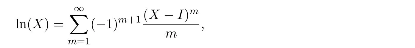
forXin a neighbourhood of the identityIofH(n).

LetEkldenotes matrix whose all entries are zero except thek-thline andl-thcolumn which is 1,then the basis of the manifoldH(n)can be given as

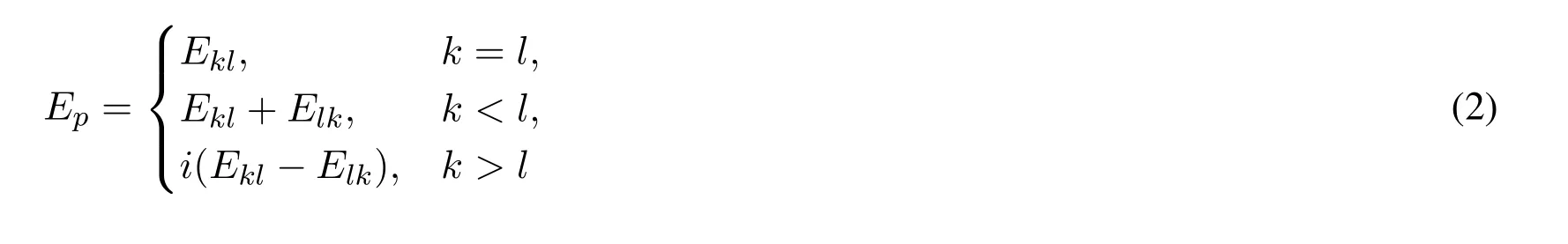
wherei2=-1,pis obtained by some rule from the pair(k,l).Hence,any positive-definite Hermitian matrixQ∈H(n)can be shown as

Definition 2.1(Duan et al.[Duan,Sun,Peng and Zhao(2013)]).Letgbe the Riemannian metric on the positive-definite Hermitian matrix manifoldH(n),forQ∈H(n)the inner product onTQH(n)can be defined as

whereM,N∈TQH(n).

Obviously,the metric defined above satisfies the fundamental properties of Riemannian metric and keeps invariant under base transformation on the tangent space.

Definition 2.2(Duan et al.[Duan,Sun and Zhang(2014);Luo and Sun(2014)]).Letγ:[0,1]→Mbe a piecewise smooth curve on manifoldM,we define the length ofγas

then the distance between any two pointx,y∈Mcan be defined as

Proposition 2.1(Duan et al.[Duan,Sun,Peng and Zhao(2013);Luo and Sun(2014)]).For the defined Riemannian metric(3)on the positive-definite Hermitian matrix manifoldH(n).We get the geodesic originating fromQalongXdirection as follows

Hence,the geodesic distance betweenQ1,Q2is shown as

According to Hopf-Rinow theorem,the positive-definite Hermitian matrix manifold is complete,which means we can always find a geodesic that connects any two pointsQ1,Q2∈H(n).

In our case,the geodesic curveγ(t)is given by

withγ(0)=x;γ(1)=yand ˙γ(0)=x1/2ln(x-1/2yx-1/2)x1/2∈H(n)then the midpoint ofxandyis defined byx?y=x1/2(x-1/2yx-1/2)x1/2and the geodesic distanced(x,y)can be computed explicitly by

whereλiare eigenvalues ofx-1/2yx-1/2.orx-1y,.

3 Solution of Algebraic Lyapunov Matrix Equation

Suppose the state of the systemX(t)is˙x(t)=Ax(t).Consider the Lyapunov function

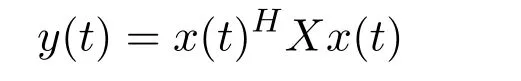
on the complex field,we have

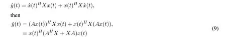
In order to make the system stable,the state Eq.(9)must be negative definite,which yields

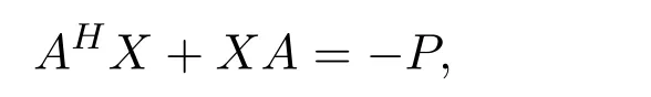
wherePis a positive-definite Hermitian matrix.

The uniqueness of the solution of Algebraic Lyapunov Eq.(1)is a well-known fact,stated below(see Davis et al.[Davis,Gravagne,Robert and Marks(2010)]):

Theorem 3.1.Given a positive-definite Hermitian matrixP＞0,there exists a unique positive-definite HermitianX＞0satisfying(1)if and only if the linear system˙x=Axis globally asymptotically stable i.e.the real part of eigenvalues ofAis less than 0.

3.1 Extended Hamiltonian Algorithm

Considering the algebraic Lyapunov Eq.(1)on the positive-definite Hermitian matrix manifold,its solution can be described as finding a positive-definite Hermitian matrixXonH(n)such that the matrix-AHX-XAis as close asP(see Fig.1).

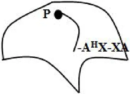
Figure 1:Geodesic distance on positive-definite hermitian matrix manifold

To describe the distance between-AHX-XAandP,we choose the geodesic distance between them as the measure,that is to say the target function is

then the optimal solution of the Eq.(1)is

Lemma 3.1(Zhang[Zhang(2004)]).Letf(X)be the scalar function of the matrixX,ifdf(X)=tr(WdX)holds,then the gradient off(X)with respect toXis

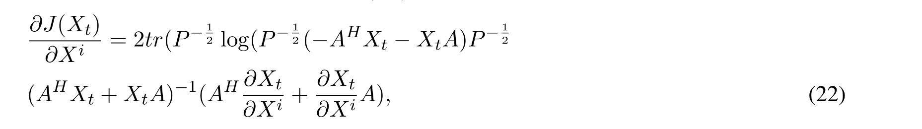
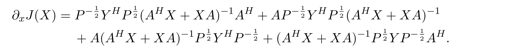
Theorem 3.2.LetJ(X)be the function in(10),then the gradient ofJ(X)with respect to the positive-definite Hermitian matrixXis

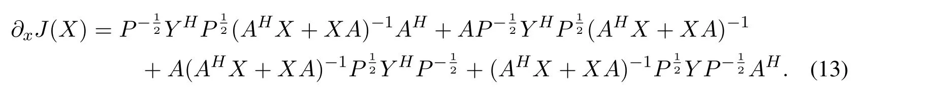
Proof of the above Theorem see the Appendix.

Theorem 3.3.On the positive definite Hermitian matrix system,if thei-th iteration matrix and direction matrix areXi,Virespectively,then(i+1)-th iteration matrix and direction matrixXi+1,Vi+1satisfy

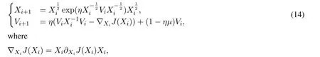
Algorithm 3.1.For the manifoldH(n)the algorithm is given as follows.HereJ(X)is the cost function(10).

1.Input initial matrixX0,initial directionV0,step sizeηand error toleranceε＞0;

2.Calculate the gradient?XiJ(Xi)by(13);

3.IfJ(Xi)＜ε,then halt;

4.UpdateX,Vaccording to(14)and go back to step 2.

巧用Flash動(dòng)畫視頻促進(jìn)文化理解。除了之前提到的這些媒體手段，大量的FLASH課件也充實(shí)著我們的音樂課堂，F(xiàn)LASH課件運(yùn)用色彩鮮艷的矢量動(dòng)畫，很好地展現(xiàn)了音樂需要表達(dá)的意境和情景，達(dá)到了音畫一體的感覺。

3.1.1 Numerical experiment

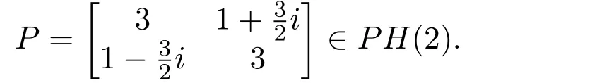
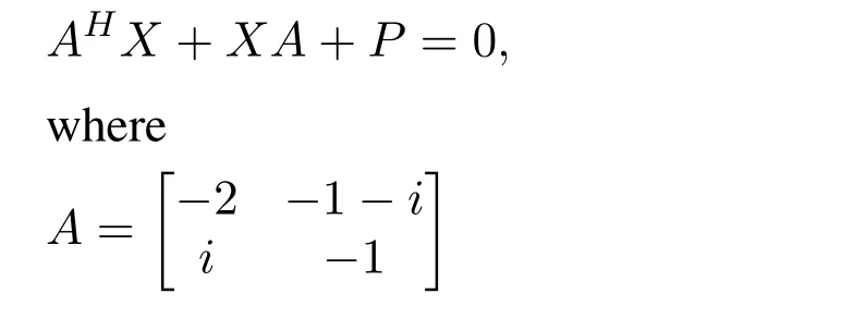
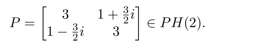
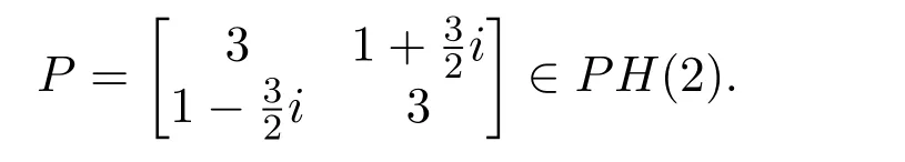
Consider the submanifoldPH(2)ofH(2)defined by:

Now we consider the algebraic Lyapunov equation on the manifold of positive-definite Hermitian matrices.

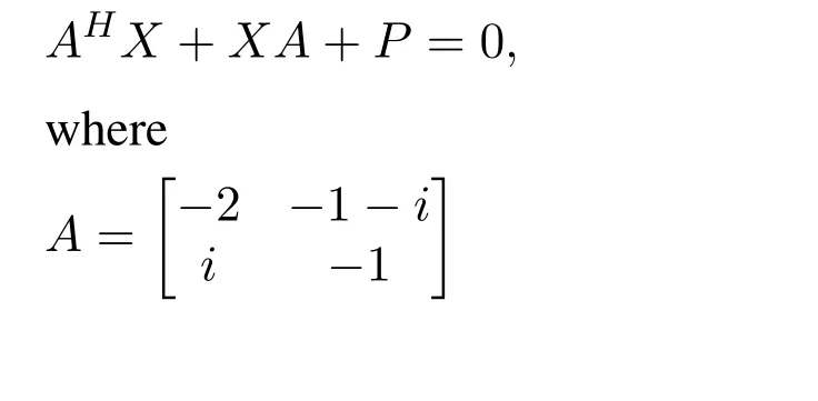
is any matrix with real part of its eigenvalues negative by Theorem 3.1,and

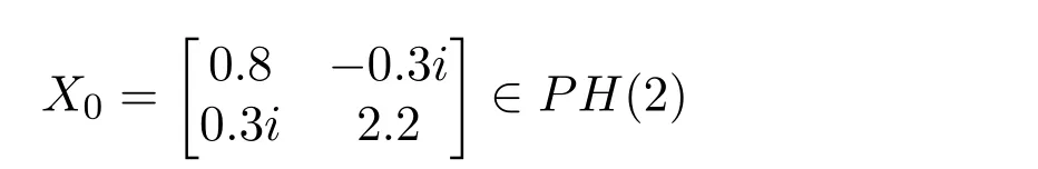
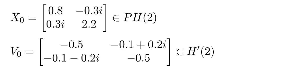
In this experiment,we choose initial guessX0and initial directionV0as

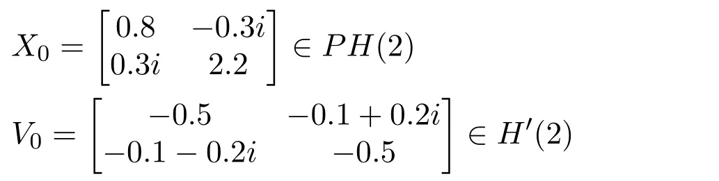
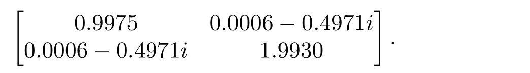
Taking the step sizeη=0.1andμ=6,then after41iterations,we obtain the optimal solution under the error toleranceε=10-3as follows,

In fact,the exact solution of(1)on the positive-definite Hermitian matrix manifold in this example is

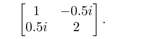
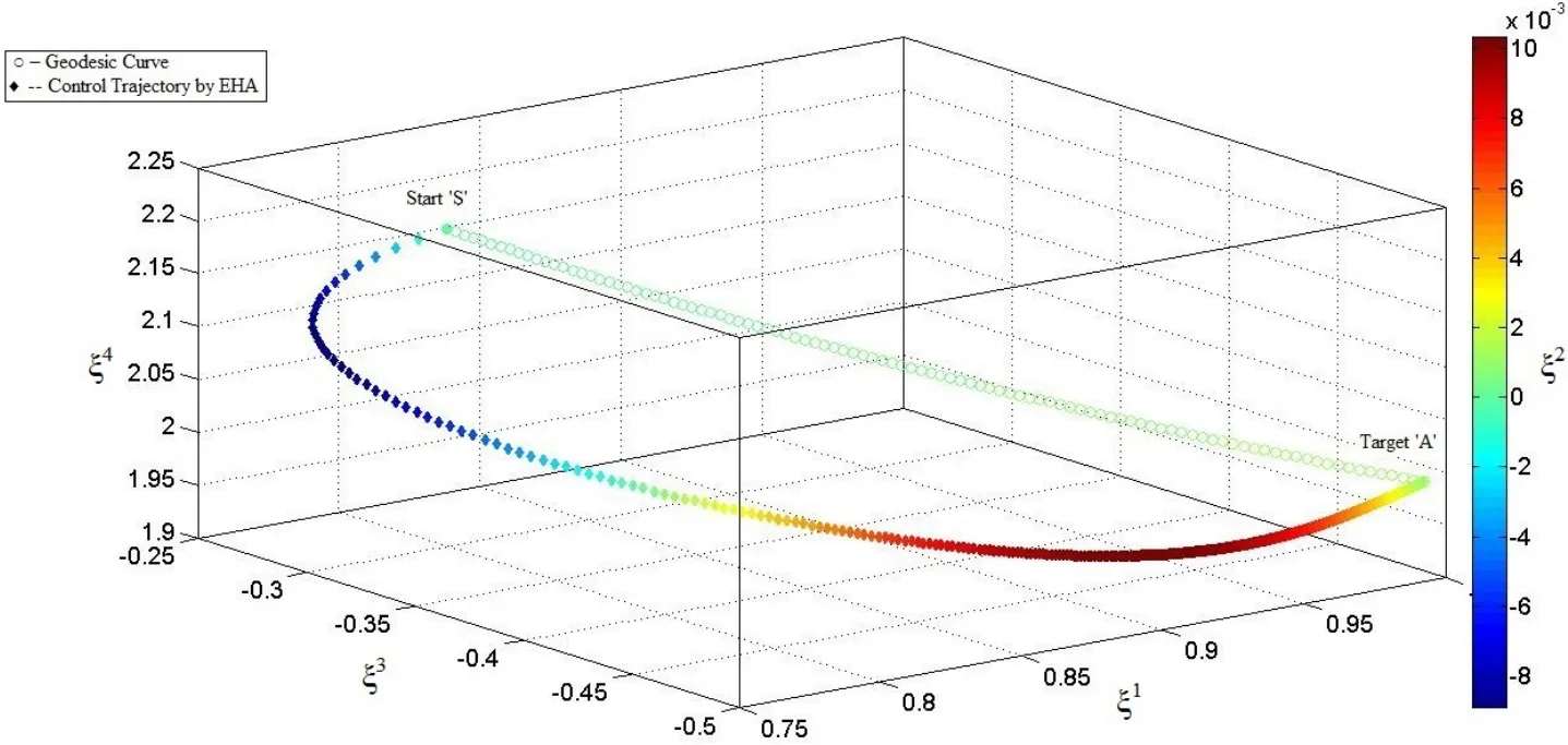
Figure 2:The optimal trajectory of EHA where η =0.1,μ =6 and ε=10-3

Futhermore,we compare the efficiency of the algorithm with different step sizes.In Fig.3,the descent curves corresponding toη=0.1,0.15,0.2show us the relation betweenJ(X)and iterations.

From the Fig.3,we can find that ifηis too small,the iterations are many and the algorithm converges slowly.However,the step size can not be too large and may result in divergence of this algorithm.Therefore,we need to adjust the step size to obtain the best convergence speed.

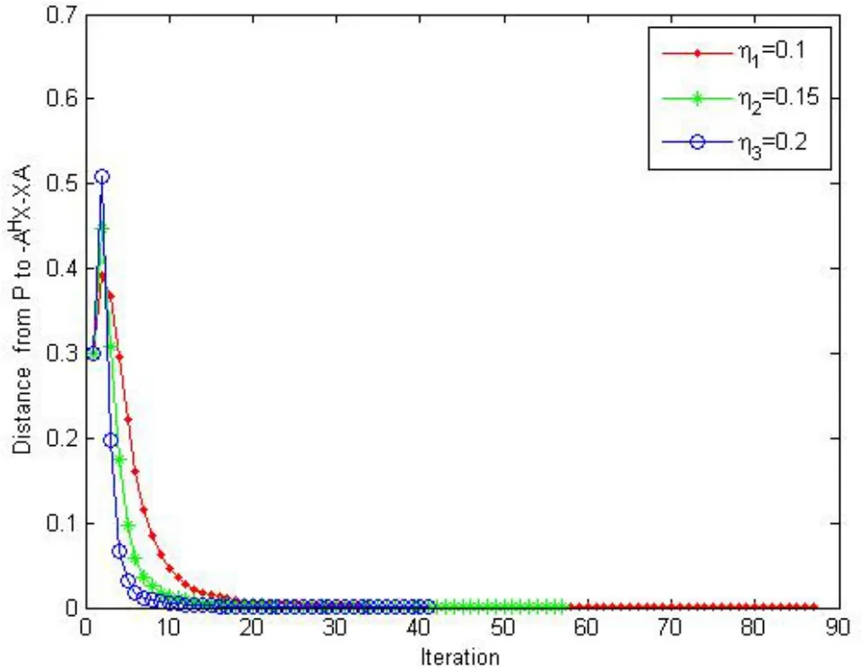
Figure 3:The efficiency of the Algorithm with different step size

3.2 Natural Gradient Algorithm

SinceH(n)is a Riemannian manifold,not a Euclidean space,therefore,it is non optimal to make use of the classical Frobenius inner product:

as a flat metric on manifoldH(n)for this geometric problem?.Moreover,since the geodesicA+t(B-A)is a negative metric for some values oft,so it is not appropriate to apply the ordinary gradient methods on the manifoldH(n)with metric(16).Observing that the geodesic is the shortest path between two points on a manifold,therefore we take geodesic distance as the cost function,denoted by:

then the optimal solution of Algebric Lyapunov equation is obtained by

As stated above,the ordinary gradient can not give the steepest descent direction of the cost functionJ(Xt)on manifoldH(n),whereas the natural gradient algorithm(NGA)does.Below we state an important Lemma,which gives the iterative step in the natural gradient algorithm.

Lemma 3.2(Amari[Amari(1998)]).LetX=(ζ1,ζ2,...ζm)∈Rmbe a parameter space on the Riemannian manifoldH(n),and consider a functionL(ζ).Then the natural gradient algorithm is given by:

whereG-1=(gij)is the inverse of the Riemannian metricG=(gij)and

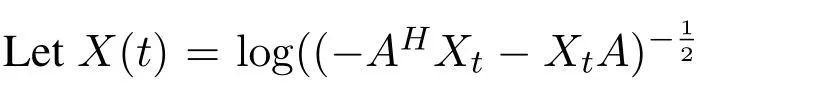
Now,we will give the natural gradient descent algorithm for the considered Eq.(1),taking the geodesic distanceJ(Xt)as the cost function and the negative of the gradient of the cost functionJ(Xt)aboutXtto give the descent direction in the iterative equation.

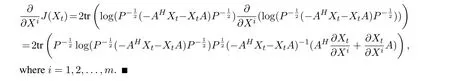
Theorem 3.4.The iteration on manifoldH(n)is given by

where the component of gradient?J(Xt)satisfies

wherei=1,2,...,m.

For Proof of above Theorem See the Appendix.

By these discussion,we present the natural gradient algorithm to find the solution of the algebraic Lyapunov Eq.(1)on the manifoldH(n)of positive-definite Hermitian matrices.

Algorithm 3.2.For the coordinateX=(ζ1,ζ2,...,ζm)of the considered manifold H(n),the natural gradient algorithm is given by;

1.SetX°=(ζ1°,ζ2°,...,ζm°)as the initial input matrix X and choose required tolerance?°＞0.

2.ComputeJ(Xt)=d2(P,-AHXt-XtA)

3.If‖?J(Xt)‖F(xiàn)＜?°,then halt.

4.Update the vectorXbyXt+1=Xt-ηG-1?J(Xt),whereXt=(ζ1t,ζ2t,...,ζmt),ηis learning rate and go back to step 2.

3.2.1 Numerical Simulations

Consider the submanifoldPH(2)ofH(2)defined by:

Now we consider the algebraic Lyapunov equation on the manifold of positive-definite Hermitian matrices:

is any matrix with real part of its eigenvalues negative by Theorem 3.1,and

In this experiment,we choose initial guessX0as

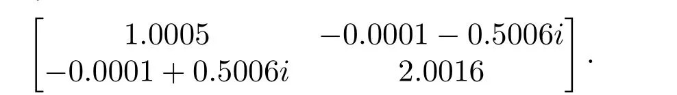
Taking the step sizeη=0.035,then after44iterations,we obtain the optimal solution under the error toleranceε=10-2as follows,

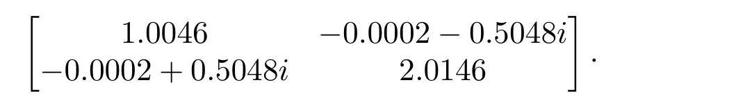
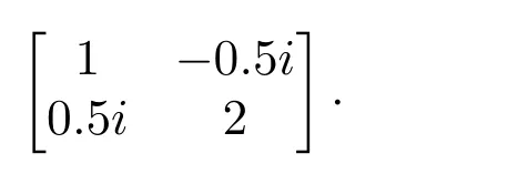
In fact,the exact solution of(1)in this example is:

In Fig.4,ζ1,ζ2,ζ3,ζ4represent coordinates of the manifoldPH(2),SandAdenote the initial matrix and the goal matrix respectively.The coordinatesζ1,ζ3,ζ4are taken along coordinate axes andζ2is represented by colour bar.The curve fromStoAshows us the optimal trajectory by NGA.Fig.4 also shows the geodesic connectingSandAobtained by(6).

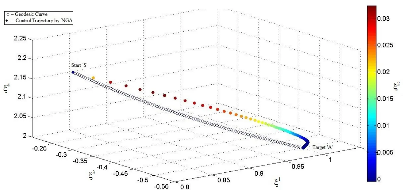
Figure 4:The optimal trajectory of NGA where η=0.035 and ε=10-2

Futhermore,we compare the efficiency of the algorithm with different step sizes.In Fig.5,the descent curves corresponding toη=0.015,0.025,0.035show us the relation betweenJ(X)and iterations.

From the Fig.5,we can find that ifηis too smaller,the iterations are many and the algorithm convergent slowly.However,the step size can not be too large,which may result in divergence in this algorithm.Therefore,we need to adjust the step size in order to obtain the best convergence speed.

3.3 Comparison of NGA and EHA

We apply the natural gradient algorithm 3.2 and extended Hamiltonian algorithm 3.1 to solve the algebraic Lyapunov Eq.(1).From the following example,we can see the efficiency of the two proposed algorithms.

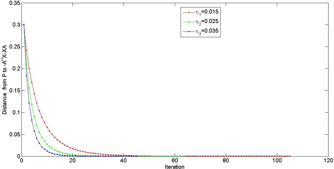
Figure 5:The efficiency of the Natural gradient Algorithm with different step size

Consider the submanifoldPH(2)ofH(2)defined by:

Now we consider the algebraic Lyapunov equation on the manifold of positive-definite Hermitian matrices.

is any matrix with real part of its eigenvalues negative by Theorem 3.1,and

In this experiment,we choose initial guessX0and initial directionV0as

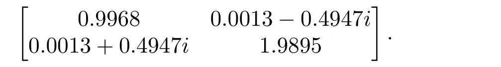
According to algorithm 3.1,we get the solution of algebraic Lyapunov equation withη=0.07,μ=4and error tolerance?=10-3as

According to algorithm 3.2,we get the solution of the algebraic Lyapunov equation withη=0.07and error tolerance?=10-3as Besides,the optimal trajectory ofX(t)from the initial input to the target matrix is shown in Fig.6.

In Fig.6,ζ1,ζ2,ζ3,ζ4represent parameters of the vectorX(t),SandAdenote the initial matrix and the goal matrix respectively.The parametersζ1,ζ2,ζ3are taken along coordinate axes andζ4is represented by colour bar.The curves fromStoAshows us the optimal trajectory ofX(t)by NGA and EHA.Fig.6 also shows the geodesic connectingSandAobtained by(6).In addition,although the trajectory of the inputX(t)given by EHA is not optimal,but the convergence is faster than NGA.

The EHA and NGA are respectively applied to get the solution of the algebraic Lyapunov equation.In particular,the behaviour of the cost function is shown in Fig.7.In early stages of learning,the EHA decreases much faster than NGA with the same learning rate.The result shows that the EHA has faster convergence speed and need 95 iterations to obtain optimal solution of Algebraic Lyapunov equation as compared to NGA which converges after 155 iterations.

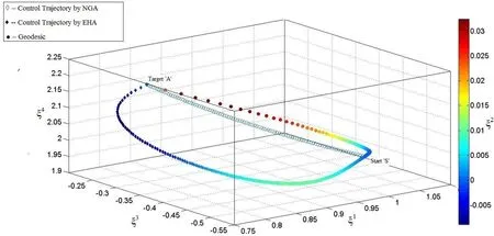
Figure 6:The optimal trajectory of X(t)by NGA and EHA where η =0.07,μ =4 and ?=10-3

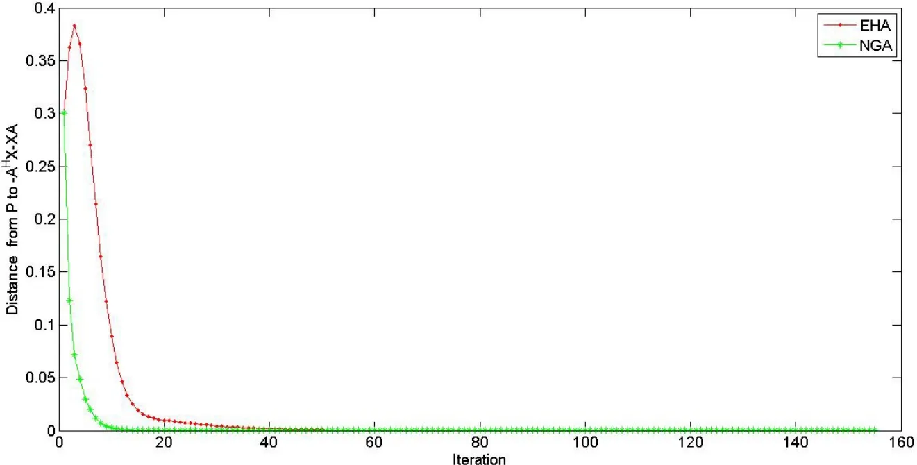
Figure 7:Comparison of convergence speed of EHA an NGA

4 Conclusion

We studied the solution of continuous algebraic Lyapunov equation by considering the positive-definite Hermitian matrices as a Riemannian manifold and used geodesic distance to find the solution.Here we used two algorithms,the extended Hamiltonian algorithm and the natural gradient algorithm to get the approximate solution of algebraic Lyapunov matrix equation.Finally,several numerical experiments give you an idea about the effectiveness of the proposed algorithms.We also show the comparison between these two algorithms EHA and NGA.Henceforth we conclude that the extended Hamiltonian algorithm has better convergence speed than the natural gradient algorithm,whereas the trajectory of the solution matrix is optimal in case of NGA as compared to EHA.

5 Appendix

Proof of Theorem 3.2

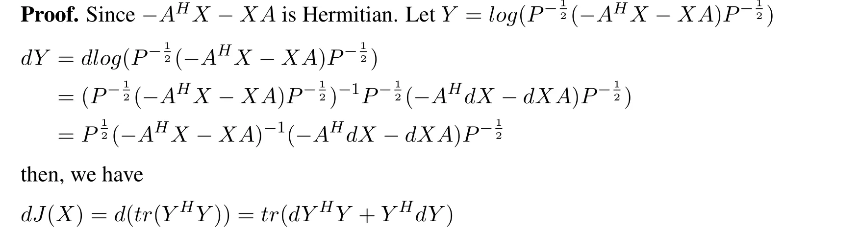
According to Lemma 4.3.1,the geodesic ofJ(X)with respect toXis

Proof of Theorem 3.4

Proof.According to above Lemma,we can get the iterative process

Acknowledgement:The authors wish to express their appreciation to the reviewers for their helpful suggestions which greatly improved the presentation of this paper.

Amari,S.(1998):Natural gradient works efficiently in learning.Neural Computation,vol.10,no.2,pp.251-276.

Amari,S.(1999):Natural gradient for over-and under-complete bases in ica.Neural Computation,vol.11,no.8,pp.1875-1883.

Amari,S.;Douglas,S.C.(2000):Why natural gradient,acoustics.Speech and Signal Processing,vol.2,pp.1213-1216.

Arif,M.S.;Zhang,E.C.;Sun,H.(2016):An information geometric algorithm for algebraic lyapunov equation on positive definite matrix manifolds.Transaction of Beijing institute of Technology,vol.36,no.2,pp.205-208.

Barbaresco,F.(2009):Interactions between symmetric cone and information geometries.Bruhat-Tits and Siegel Spaces Models for High Resolution Autoregressive Doppler Imagery,ETVC,vol.5416,pp.124-163.

Brown,M.;Harris,C.(1994):Neurofuzzy Adaptive Modelling and Control.Prentice Hall New York.

Cafaro,C.(2008):Information-geometric indicators of chaos in gaussian models on statistical manifolds of negative ricci curvature.International Journal of Theoretical Physics,vol.47,no.11,pp.2924-2933.

Chein,S.L.(2014): A sliding mode control algorithm for solving an ill-posed positive linear system.Computers,Materials&Continua, vol. 39, no. 2, pp. 153-178.

Cohn,S.E.;Parrish,D.F.(1991):The behavior of forecast covariances for a kalman filter in two dimensions.Neural Computation,vol.119,no.8,pp.1757-1785.

Datta,B.N.(2004):Numerical Methods for Linear Control Systems.Elsvier Academic-Press.

Davis,J.M.;Gravagne,I.A.;Robert,J.;Marks,I.(2010):Algebraic and dynamic lyapunov equations on time scales.42nd South Eastern Symposium on System Theory at University of Texas,USA,pp.329-334.

Deng,Y.B.;Bai,Z.Z.;Gao,Y.H.(2006):Iterative orthogonal direction methods for hermitian minimum norm solutions of two consistent matrix equations.Numer.Linear.Alg.Appl.,vol.13,no.10,pp.801-823.

Duan,X.;Sun,H.;Peng,L.;Zhao,X.(2013):A natural gradient descent algorithm for the solution of discrete algebraic lyapunov equations based on the geodesic distance.Applied Mathematics and Computation,vol.219,no.19,pp.9899-9905.

Duan,X.;Sun,H.;Zhang,Z.(2014):A natural gradient algorithm for the solution of lyapunov equations based on the geodesic distance.Journal of Computational Mathematics,vol.32,no.1,pp.93-106.

Fiori,S.(2011):Extended hamiltonian learning on riemannian manifolds,theoretical aspects.IEEE Transactions on Neural Networks,vol.22,no.5,pp.687-700.

Fiori,S.(2012):Extended hamiltonian learning on riemannian manifolds,numerical aspects.IEEE Transactions on Neural Networks and Learning Systems,vol.23,no.1,pp.7-21.

Golub,G.H.;Nash,S.;Vanloan,C.(1979):A hessenberg-schur method for the problemax+xb=c.IEEE Transactions on Automatic Control,vol.24,no.6,pp.909-913.

Jbilou,K.(2010): Adi preconditioned krylov methods for large lyapunov matrix equations.Linear Algebra & Its Applications, vol. 432, no. 10, pp. 2473-2485.

Li,J.R.;White,J.(2002):Low-rank solution of lyapunov equations.SIAM J.Matrix Appl.,vol.24,no.1,pp.260-280.

Luo,Z.;Sun,H.(2014):Extended hamiltonian algorithm for the solution of discrete algebraic lyapunov equations.Applied Mathematics and Computation,vol.234,pp.245-252.

Moakher,M.(2005):A differential geometric approach to the geometric mean of symmetric positive-definite matrices.SIAM Journal on Matrix Analysis and Applications,vol.26,no.3,pp.735-747.

Moakher,M.;Batcherlor,P.G.(2006):Symmetric Positive-Definite Matrices:From Geometry to Applications and Visualizatin,Visualization and Processing of Tensor Fields.Springer.

Ran,A.C.M.;Reurings,M.C.B.(2004):A fixed point theorem in partially ordered sets and some applications to matrix equations.Proc.Am.Math.Soc.,vol.132,pp.1435-1443.

Su,Y.F.;Chen,G.L.(2010):Iterative methods for solving linear matrix equation and linear matrix system.Numer.Linear.Alg.Appl.,vol.87,no.4,pp.763-774.

Vandereycken,B.;Vandewalle,S.(2010):A riemannian optimization approach for computing low-rank solutions of lyapunov equations.SIAM J.Matrix Appl.,vol.31,no.5,pp.2553-2579.

Zhang,X.D.(2004):Matrix Analysis and Application.Springer,Beijing.