MODIFIED LAVRENTIEV REGULARIZATION METHOD FOR THE CAUCHY PROBLEM OFHELMHOLTZ-TYPE EQUATION

Zhang Hong-wu,Zhang Xiao-ju

(1.School of Mathematics and Information Science,North Minzu University,Yinchuan 750021,China)

(2.Center of Faculty Development,North Minzu University,Yinchuan 750021,China)

Abstract:In this paper,a Cauchy problem of Helmholtz-type equation with nonhomogeneous Dirichlet and Neumann datum is researched.We establish the result of conditional stability under an a-priori assumption for exact solution.A modified Lavrentiev regularization method is used to overcome its ill-posedness,and under an a-priori and an a-posteriori selection rule for the regularization parameter we obtain the convergence result for the regularized solution,the corresponding results of numerical experiments verify that the proposed method is stable and workable，this work is an extension on the related research results of existing literature in the aspect of regularization theory and algorithm for Cauchy problem of Helmholtz-type equation.

Keywords:ill-posed problem;Cauchy problem;Helmholtz-type equation;modified Lavrentiev method;convergence estimate

1 Introduction

In some practical and applied fields,such as Debye-Huckel theory,implicit marching strategies of the heat equation,the linearization of the Poisson-Boltzmann equation,Helmholtz-type equation had many important applications,see[1–4],etc.In the past century,the direct problem for it caused the extensive attention and was researched widely.However,in some science research areas,the data of the entire boundary can not be acquired,we only can measure the one on a part of the boundary or at certain internal points of one domain,which is called as the inverse problem for the Helmholtz-type equation.This paper studies the Cauchy problem of Helmholtz-type equation

wherek＞0 is the wave number.In view of the linear property of(1.1),it can be divided into two problems,i.e.,the Cauchy problem with nonhomogeneous Dirichlet data

and the Cauchy problem with inhomogeneous Neumann data

it is easily to be know that the solution of problem(1.1)can be expressed asw=u+v.Then,we only need to research problems(1.2)and(1.3),respectively.

Problems(1.2)and(1.3)are both the ill-posed problems in the sense that a small disturbance on the Cauchy datum can lead to an tremendous error in the solution[5–7],so some regularization techniques must be carried to overcome the ill-posedness and stabilize numerical calculations(see some regularization strategies in[8,9]).In the past years,we find that many scholars have considered the Cauchy problem of Helmholtz-type equation and proposed some efficient regularized methods and numerical techniques,such as quasi-reversibility type method[10–14], filtering function method[15],iterative method[16],mollification method[17,18],spectral method[19,20],alternating iterative algorithm[21,22],modified Tikhonov method[20,23],Fourier method[12,24],novel trefftz method[25],weighted generalized Tikhonov method[26],and so on.

In this paper,we firstly establish the conditional stabilities for problems(1.2),(1.3),and then construct a kind of modified Lavrentiev regularization method to solve these two problems.In our work,we shall derive some a-priori and a-posteriori convergence results of H?lder type for our regularization solutions,and give an a-posteriori selection rule for the regularization parameter which is relatively rare in solving the Cauchy problem of Helmholtztype equation.The work is an extension and supplement for the existing ones.

The paper is organized as follows.In Section 2,we derive the conditional stabilities of(1.2)and(1.3).Sections 3 constructs the modified Lavrentiev regularization methods,Sections 4 states some preparation knowledge.In Section 5,the a-priori and a-posteriori convergence estimates of sharp type are established.Some numerical results are shown in Section 6.The corresponding conclusions and discussions are drawn in Section 7.

2 Conditional Stability

We know that the Cauchy problem of the Helmholtz-type equation is ill-posed in the sense of Hadamard that the solution(if it exists)discontinuity depends on the given Cauchy data.Under an additional condition,a continuous dependence of the solution on the Cauchy data can be obtained,which is so-called conditional stability[27–29].In this section,under an a-priori bound assumption for exact solutions,we give the conditional stabilities of problems(1.2)and(1.3).Forγ≥1/2,q＞0,we define

here,〈·,·〉denotes the inner product inis the eigenfunctions inL2(0,π),and the norm ofis defined as

Applying the method of variables separation,the solutions of(1.2)and(1.3)respectively can be expressed as

Theorem 2.1LetE＞0,u(T,x)satisfy an a-priori bound condition

then for each fixed 0＜y≤T,it holds that

whereK=1+k2.

ProofNote that,for 0＜y≤T,n≥1,n2+k2≥1+k2,then from(2.3),(2.5)and Hlder inequality,we have

Theorem 2.2Suppose thatv(T,x)satisfies the a-priori condition

then for the fixed 0＜y≤T,we have

ProofForn≥1,wenotice that sinh,sinhfrom(2.4),(2.7)andH¨older inequality,we have

From the inequality above,we can derive the conditional stability result(2.8).

3 Regularization Method

From(2.3),(2.4),we know that coshare unbounded asntends to in finity,so problems(1.2),(1.3)are both ill-posed,i.e.,the solutions do not depend continuously on the Cauchy datumφandψ.In order to restore the stability of solutions given by(2.3)and(2.4),we need eliminate the high frequencies of two functions to construct the regularized solutions for(1.2),(1.3).

3.1 Regularization Method for Problem(1.2)

We adopt the similar idea in[30],then problem(1.2)can be equivalently expressed as the following operator equation

Let us introduce the Hilbert scale(Hμ)μ∈R+according toandis the norm inHμ.Forγ≥1/2,we construct a generalized Tikhonov regularization solutionby solving the minimization problem

here,φδ(x)=uδ(0,x)denotes the noisy data,δis measured error bound,andαplays the role of regularization parameter,u*∈L2(0,π)is the reference element(initial guess).Henceis the solution of Euler equation

of the functionalJα.Note that the operatorA1(y)is a monotone compact operator,i.e.,〈A1(y)u(y,·),u(y,·)〉L2(0,π)≥0,andA1(y)is compact with dimR(A1(y))=∞,then(3.1)is an ill-posed problem of type II in sense of Nashed[31](also see[32]).So adopting the similar idea with[33],we can replaced(3.3)by the simpler regularized equation below

which is a Lavrentiev-type method(see[34]),i.e.,

We know that the ordinary Lavrentiev method[35]is characterized by(3.5),andis replaced byαI.

Settingq＞0,now we firstly replace coshby coshin the left side of(3.5),and then express it a singularly perturbed form,it can be obtained a modified Lavrentiev method for solving linear ill-posed problem(3.1).The regularized equation can be written as

We take the reference element(initial guess)u*≡0 and solve equation(3.6),then the regularized solution can be written as

3.2 Regularization Method for Problem(1.3)

As in Subsection 3.1,we also can convert(1.3)into the operator equation

Note thatA2(y):L2(0,π)→L2(0,π)also is a monotone and compact operator with dimR(A(y))=∞,then(3.9)is an ill-posed problem of type II in sense of Nashed.Similar with the process in Subsection 3.1,forγ≥1/2,we construct a generalized Tikhonov regularization solutionby solving the minimization problem

of the functionalIβ.Since the operatorA2(y)is a monotone compact operator,we can replaced(3.11)by the simpler regularized equation(Lavrentiev-type method)

i.e.,

Letq＞0,we replace sinhby sinhin the left side of(3.13),and express it a singularly perturbed form,we can obtain a modified Lavrentiev method for solving ill-posed problem(3.9).The regularized equation can be written as

We also choose the initial guessv*≡0 and solve equation(3.14),the regularized solution can be expressed as

4 Preparation Knowledge

Letα,β,q,k＞0,γ≥1/2,K=1+k2,n≥1,for each fixed 0＜y≤T+q,we define the functions

and

We also require the following Lemma 4.1 which is given and proven in the reference[36].

Lemma 4.1If 0≤r≤s＜∞,0,andν＞0,then

where

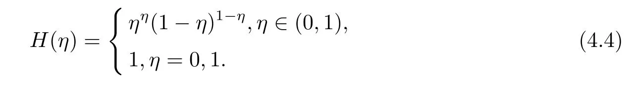
Theorem 4.2Letα＞0,H1(n)is defined by(4.1),then for each fixed 0＜y≤T+q,we have

ProofApply Lemma 4.1 withand fromH(η)≤1,we have

29. Pigeon: Pigeons are birds having a heavy body and short legs. They can be wild or domesticated86 (WordNet). Since pigeons are often domesticated birds, they are associated with the desire to return home in dream interpretations88.

Theorem 4.3Letβ＞0,H2(n)is defined by(4.2),then for the fixed 0＜y≤T+q,it holds that

Pr oofWe takein Lemma 4.1,and fromH(η)≤1,inequality(4.6)can be derived.

5 Convergence Estimate

In this section,under the a-priori and a-posteriori selection rules for the regularization parameter we derives the convergence estimate for modified Lavrentiev regularization method.

5.1 Convergence Estimate for the Method of Problem(1.2)

5.1.1 A-Priori Convergence Estimate

Theorem 5.1Letube the exact solution of problem(1.2)given by(2.3),defined by equation(3.7)is the regularization solution,the measured dataφδsatisfies(3.8).If the exact solutionusatisfies

and the regularization parameterαis chosen as

then for fixed 0＜y≤T,we have the convergence estimate

ProofDenoteuαbe the solution of problem(3.7)with exact dataφ.We use the triangle inequalities,then

For 0＜y≤T+q,asn≥1,from(3.7),(4.5),(3.8),we note that

On the other hand,by(2.3),(3.7),(4.5),(5.1),we have

Finally,we can complete the proof by using(5.4),(5.5),(5.6)and(5.2).

5.1.2 A-Posteriori Convergence Estimate

In Theorem 5.1,we select the regularization parameterαby an a-priori rule(5.2),which needs the a-priori boundEof exact solution.However,in practice the a-priori boundEgenerally can be not known easily.In the following we adopt a kind of the a-posteriori rule to selectα,this method need not know the a-priori bound for exact solution,and the regularization parameterαdepend on the measured dataφδand measured error boundδ.On the reference that describes the a-posteriori rule in selecting the regularization parameter,we can see[37],etc.

We select the regularization parameterαby the following equation

hereτ＞1 is a constant.We need two lemmas that will be used in deriving the a-posteriori convergence estimate.

Lemma 5.2Letthen we have the following conclusions

(a)ρ(α)is a continuous function;

(d)Forα∈(0,+∞),ρ(α)is a strictly increasing function.

ProofIt can be easily proven by setting

Lemma 5.2 indicates that there exists a unique solution for(5.7)if‖φδ‖ ＞τδ＞0.

Lemma 5.3For the fixedτ＞1,the regularized solution(3.7)combining with aposteriori rule(5.7)determine that the regularization parameterα=α(δ,φδ)satisfies

ProofFrom(5.7),there holds

and

from(5.9),(5.10),we get thatThe proof is completed.

Theorem 5.4Letugiven by(2.3)be the exact solution of problem(1.2),defined by(3.7)is the regularization solution,the measured dataφδsatisfies(3.8).If the exact solutionusatisfies a priori bound(5.1),the regularization parameter is chosen by a-posteriori rule(5.7),then for each fixed 0＜y≤T,we have the convergence estimate

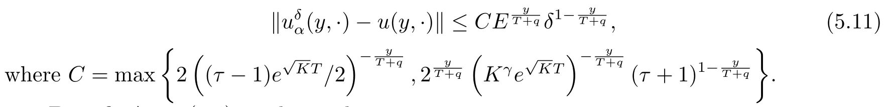
ProofAs in(5.4),we know that

By(5.5)and Lemma 5.3,we get

Now we give the estimate for the second term of(5.12).For fixed 0＜y≤T,note that

using(3.8),(5.7),(5.14),we can obtain that

Meanwhile,according to the definition in(2.2)and a-priori condition(5.1),we have

then,by the condition stability result(2.6),it can be obtained that

Finally,combining(5.13)with(5.17),we can obtain the convergence estimate(5.11).

5.2 Convergence Estimate for the Method of Problem(1.3)

5.2.1 A-Priori Convergence Estimate

Theorem 5.5Letvgiven by(2.4)be the exact solution of problem(1.3),defined by(3.15)is the regularization solution,the measured dataψδsatisfies(3.16).If the exact solutionvsatisfies

and the regularization parameterβis chosen as

then for fixed 0＜y≤T,we have the following convergence estimate

whereC1is given in Theorem 4.3.

ProofDenotevβbe the solution defined by(3.15)with exact dataψ.Using the triangle inequality,we get that

For 0＜y≤T+q,asn≥1,sinhfrom(3.15),(4.6),(3.16),we note that

On the other hand,by(2.4),(3.15),(4.6),(5.18),we have

From(5.19),(5.21),(5.22),(5.23),the convergence result(5.20)can be derived.

5.2.2 A-Posteriori Convergence Estimate

We findβsuch that

hereτ＞1 is a constant.

Lemma 5.6Letthen we have the following conclusions

(a)?(β)is a continuous function;

(d)Forβ∈(0,+∞),?(β)is a strictly increasing function.

ProofIt can be easily proven by setting

Lemma 5.6 means that there exists a unique solution for(5.24)if‖ψδ‖＞τδ＞0.

Lemma 5.7For the fixedτ＞1,the regularization solution(3.15)combining with a-posteriori rule(5.24)determine that the regularization parameterβ=β(δ,ψδ)satisfies

ProofFrom(5.24),there holds

and

combing with(5.26)and(5.27),we otain that

Theorem 5.8Letvgiven by(2.4)be the exact solution of problem(1.3),defined by(3.15)is the regularization solution,the measured dataφδsatisfies(3.16).If the exact solutionvsatisfies a priori bound(5.18),and the regularization parameter is chosen by a-posteriori rule(5.24),then for fixed 0＜y≤T,we have the convergence estimate

where

C1is given in Theorem 4.3.

ProofNotice that

By(5.22)and Lemma 5.7,we get

Below,we do the estimate for the second term of(5.29).For fixed 0＜y≤T,we have

using(3.16),(5.24),(5.31),we can obtain

Meanwhile,according to the definition in(2.2)and a-priori bound condition(5.18),we have

then,by the condition stability result(2.8),we can get that

Finally,combining(5.30)with(5.34),we can obtain the convergence estimate(5.28).

6 Numerical Experiments

In this section,we use numerical experiment to verify the efficiency of our method.For the simplification,we only investigate the numerical efficiency of the regularization method for(1.2),which is similar with the case of inhomogeneous Neumann data(1.3).

ExampleWe can verify thatis the exact solution of problem(1.2).We take the Cauchy dataφ(x)=u(0,x)=sin(x).Denoteas the step size for variablex,x?=?Δxas the nodes in[0,π]for?=0,1,2,···,N,and choose the measured data asφδ=φ+εrandn(size(φ)),whereφis a(N+1)×1 dimension vector,εis the noisy level,the function randn(·)generates arrays of random numbers whose elements are normally distributed with mean 0 and standard deviation 1,randn(size(φ))returns an array of random entries that is of the same size asφ.The bound of measured errorδis calculated in the sense of the root mean square error

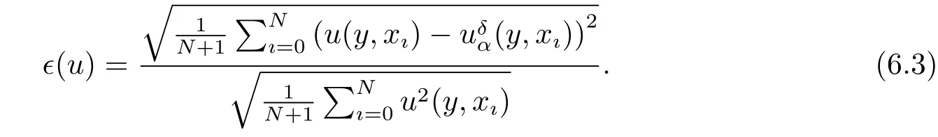
For each 0＜y≤1,the regularization solutionis computed by(3.7)forn=1,2,···,M,and the relative root mean square error is computed by

Since the a-priori boundEis generally difficult to be obtained in practice,we only give the numerical results by the a-posteriori selection rule(5.7)for the regularization parameterα,hereαis found by the Matlab command fzero,and we takeτ=1.1.

Fork=0.5,1.5,γ=2,q=0.5,the relative root mean square errors for various noisy levelεare presented in Tables 6.1–6.2.Fork=0.5,1.5,takingε=0.01,q=0.5,we also compute the corresponding errors to investigate the influence ofγon numerical results,which are shown in Tables 6.3–6.4.Fork=0.5,1.5,takingε=0.01,γ=2,we calculate the errors to investigate the influence ofqon numerical results,the results are shown in Tables 6.5–6.6.

From Tables 6.1–6.6,we observe that our method is stable and feasible.From Tables 6.1–6.2,we see that numerical results become better asεgoes to zero,which verifies the convergence of our method in practice.Tables 6.3–6.4 show that,for the sameε,q,the error decreases asγbecomes large.Tables 6.5–6.6 indicate that,for the sameε,γ,numerical results become well asqincreases.Then,in order to guarantee to obtain the satis fied calculational result,we should choose the parameterγ,qas a relative large positive number,this conclusion are coincident with the expression of the regularization solution(3.7)and the convergence result(5.11).

Table 6.1 k=0.5,γ=2,q=0.5,the relative root mean square errors for various noisy level ε at y=0.6,1

Table 6.2 k=1.5,γ=2,q=0.5,the relative root mean square errors for various noisy level ε at y=0.6,1

Table 6.3 k=0.5,q=0.5,ε=0.01,the relative root mean square errors for various γ at y=0.6,1

Table 6.4 k=1.5,q=0.5,ε=0.01,the relative root mean square errors for various γ at y=0.6,1

7 Conclusion and Discussion

The article researches a Cauchy problem of the Helmholtz-type equation with nonhomogeneous Dirichlet and Neumann datum.For problems(1.2)and(1.3),we respectively give the conditional stability estimate under an a-priori bound assumption for exact solution.One modified Lavrentiev method is constructed to solve these two problems,and some convergence results of H?lder type for our method are derived under an a-priori and an a-posteriori selection rule for the regularization parameter,respectively.We also verify the practicability of this method by making the corresponding numerical experiments.

Table 6.5 k=0.5,γ=2,ε=0.01,the relative root mean square errors for various q at y=0.6,1

Table 6.6 k=1.5,γ=2,ε=0.01,the relative root mean square errors for various q at y=0.6,1

It should be pointed out that the proposed method also can be used to solve the Cauchy problem of elliptic equation in cylindrical domain.However this method can not be applied to deal with some other problems in more general domains,which is a deficiency of this article.In addition,in the procedure of the computation,we need to choose the suitable parameters which include the regularization parameterα,positive integerNand positive numbersγ,q.We choose the parametersN,γandqby using the a-priori method,but not to consider the a-posteriori rule for them.It is well know that the selection of the parameter is a sensitive and widespread concerned issue in the inverse problems,their values often can influence the numerical computation effect directly,so it is necessary to consider the a-posteriori selection rule for the parametersN,γandqin future works.