Solving numerically the 2D inverse heat conduction problem based on the variable limit integral method

ZHANG Yan, FENG Lixin

(School of Mathematical Sciences, Heilongjiang University, Harbin 150080, China)

Abstract: Consider a 2D inverse heat conduction problem of determining the initial temperature from the temperature at the final time T>0. For the problem, an inversion method is constructed based on the regularization technique and the SOR iteration. At each iterative step, the direct problem is solved by using the proposed variable limit integral method. Numerical experiments show that this method is valid.

Keywords: inverse problem; heat conduction equation; regularization; SOR iteration; variable limit integral method

0 Introduction

Let Ω=[0,π]×[0,π]?R2. Consider the following initial boundary value problem for 2D heat conduction equation:

(1)

whereg(x1,x2) is the exact initial temperature and satisfiesg(x1,x2)|?Ω=0. The solutionu(x1,x2;t) for the direct problem (1) can be obtained by the eigen-system {un(x1,x2),λn} of the Laplace operator. That is

(2)

with the coefficients

whereun(x1,x2)andλnare, respectively, thenth orthonormalized eigenfunction and eigenvalue of

However, our aim is to study the inverse problem related to (1). The inverse problem is to find the initial temperatureu(x1,x2;0)=g(x1,x2) from the given measured datau(x1,x2;T)at the final time. For the inverse heat conduction problem, there have been many researches, see the references [1-10].

In this paper, we propose an inversion method which incorporates Tikhonov regularization technique with the SOR iteration. At each iterative step, we solve the direct problem by using the variable limit integral method developed in the paper. The variable limit integral method incorporates the finite difference method with the finite volume method. Its basic idea is to make the original partial differential equation to be an integral equation by a certain number of integrations in the independent variables (spatial or time). The goal is that the integral equation no longer contains the derivative item of the unknown function. In the integral equation, the interpolation function (for example, Lagrange interpolation) is appropriately chosen to establish a discrete scheme, refer to the references [11-14].

This paper is organized as follows. In Section 1, we analyze the ill-posedness of the inverse problem and present an inversion method which depends on the numerical solution to the direct problem (1). In Section 2, the numerical scheme of direct problem is given by utilizing the variable limit integral method, and its stability is discussed. In Section 3, some numerical examples are proposed to show the effectiveness of the proposed method. Finally, a brief conclusion is presented in Section 4.

1 The ill-posedness and regularization for 2D inverse heat conduction problem

For the direct problem (1), we define an operatorB:

Bg(x1,x2)=u(x1,x2;T), forg(x1,x2)∈L2(Ω)

(3)

Then we know from (2) that

(4)

with the kernel function

If we assume thatu(x1,x2;t) is a known function, we can get

(5)

Theoretically,g(x1,x2)can be uniquely determined by (5) for givenu(x1,x2;T). Nevertheless, the computation procedure is unstable due to the unboundedness of operatorB-1. In fact, the error in the solutiong(x1,x2) amplifies exponentially for this inverse problem from

(6)

(see reference [2]). In other words, the drastic change of error for solutiong(x1,x2) may be caused by a small error atu(x1,x2;T). Hence the inverse problem is an ill-posed problem.

The exact solution of (3) is denoted asg*(x1,x2) in the sequel for exact datau(x1,x2;T), i.e.,Bg*(x1,x2)=u(x1,x2;T). However, we can just get the approximate valueuε(x1,x2;T) ofu(x1,x2;T) in practice, and they satisfy

‖uε(x1,x2;T)-u(x1,x2;T)‖L2(Ω)≤ε

where the error levelε>0 is known. Our goal is to determine the approximate valuegε(x1,x2) ofg*(x1,x2) stably fromuε(x1,x2;T)by using a regularization technique. Define the Tikhonov functional inL2(Ω)

(7)

(8)

If the regularized parameterαis chosen such that

rn=Bu(x1,x2;T)-(αgn+B2gn)

(9)

g0arbitrary,gn=gn-1+βnrn-1,n≥1

(10)

(11)

whereβnis obtained by minimizing ‖rn‖ because of

rn=Bu(x1,x2;T)-(α+B2)(gn-1+βnrn-1)=rn-1-βn(α+B2)rn-1

From (9)～(11), it is easy to see that the generation ofrnandβnneeds to solve the direct problem four times at each iteration step, that is, which needs to solveBgn,B2gn,Brn,B2rn. Therefore, an effective numerical scheme for solving direct problem (1) should be constituted. The explicit variable limit integral method will be proposed in Section 2.

2 The variable limit integral method for direct problem (1)

2.1 Construction of numerical scheme

We integrate two sides of differential equation (1) on the control region Ω1=[xa,xb]×[ya,yb]×[tn,tn+1], wherexa,xb,ya,yb∈[0,π] andtn,tn+1∈(0,T]. It is easy to get that

(12)

Then both sides of equation (12) are integrated on the control region Ω1=[xi-ε1,xi]×[xi,xi+ε2]×[yj-ε3,yj] ×[yj,yj+ε4] forxa,xb,ya,ybrespectively, and we have

(13)

whereε1,ε3,ε2andε4are the variable limit factors that control the size of integral regions. Therefore, the differential equation (1) is completely transformed into the integral equation (13).

Now we choose Lagrange interpolation to approximate integrand of (13) near point (xi,yj;tn), i.e.,

whereR(x,y;t) is the truncation error. In addition, letε1=ε2=ε3=ε4=h. Thus we get

(14)

(15)

(16)

whereR1,R2andR3are truncation errors. Their expressions are

respectively.

Substituting (14)～(15) into (13), omitting the truncation errorsR1,R2, andR3simplifying, we get the numerical scheme, i.e.,

2.2 Stability analysis

vn+1((h2-12τ)(e-i(αh+βh)+ei(-αh+βh)+ei(αh-βh)+ei(αh+βh))+(10h2-48τ)(e-iαh+e-iβh+eiαh+eiβh)+100h2+240τ)
=vn((h2+12τ)(e-i(αh+βh)+ei(-αh+βh)+ei(αh-βh)+ei(αh+βh))+(10h2+48τ)(e-iαh+e-iβh+eiαh+eiβh)+100h2-240τ)

(18)

Letr=h2/τ∈R+. Simplifying equation (18), the growth factor of numerical scheme (17) can be obtained

The difference scheme (17) is stable if and only if |λ|2≤1, this is, |G2|2-|G1|2≤0. Computing directly |G1|2and |G2|2, we have

Sequentially,

(19)

The equation (19) can be enlarged, i.e.,

Hence, the numerical scheme (17) is always stable.

3 Numerical experiments

To illustrate the efficiency of the proposed method, we give an example. Take the exact initial temperatureg(x,y)=sin(x)sin(y), ?(x,y)∈Ω and the guessed temperatureg0(x,y)=-0.5x(π-x)y(π-y) that is used as the initial value of iteration. Such two functions are shown in Fig.1. Obviously, the guessed temperature is quite different from the exact initial temperature. For the direct problem, we know the exact solutionu(x,y;t)= sin(x)sin(y)e-2t.

In numerical experiments, we takeT=0.005,α=0.000 1,M=32 andN=32.For testing the stability of our inversion method, we give the perturbation foru(x,y;T) at nodal points (xi,yj)=(h,jh) with the form

uε(xi,yj;T)=u(xi,yj;T)+εrand(·)

where the function rand(·) generates uniformly distributed random numbers distributed between 0 and 1. For different parameters, the inversion results are shown in the following figures and tables. Additionally, the relative error is measured by ‖·‖L2.

Table 1 Solutions of the direct problem for M=N=32

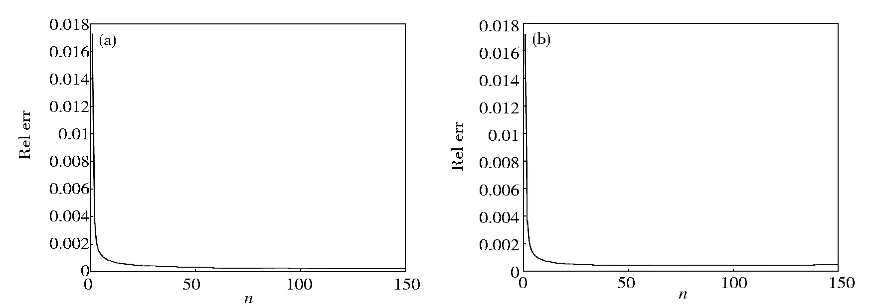
Fig.2 presents the numerical solutions and the exact solutions of direct problem. These solutions are listed in Table 1. It is obvious that the numerical scheme of direct problem is satisfactory. From Table 2, it can be observed that the inversion results are satisfactory for different perturbation. Table 3 shows the efficiency of inversion for different iteration timesnandε. The numerical convergence of reconstruction can be seen from relative error curves (Fig.4).

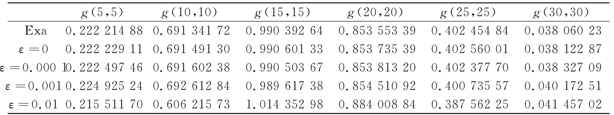
Table 2 Reconstructions of the inverse problem for(M,N,α,n)=(32,32,0.000 1,150)

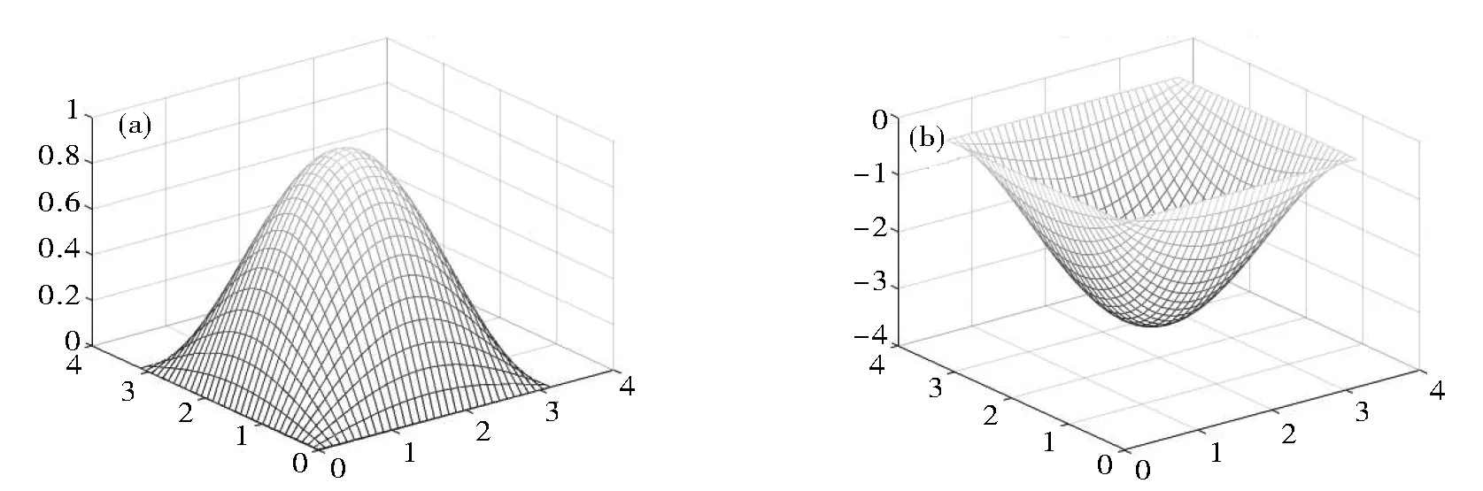
Fig.1 Initial temperature: (a) exact temperature; (b) guessed temperature

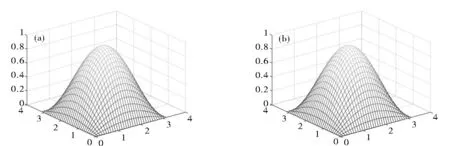
Fig.2 Solutions of the direct problem: (a) exact solution; (b) numerical solution

Fig.3 Reconstructions of the inverse problem: (a)ε=0; (b)ε=0.001; (c)ε=0.01

4 Conclusions

The inversion method for the 2D inverse heat conduction problem, which takes advantage of the Tikhonov regularization technique, the SOR iteration and the variable limit integral method, is introduced. The stability of the approximate solution is guaranteed by the Tikhonov regularization. The SOR iteration reduces the computational cost for solving Euler equation corresponding to the Tikhonov functional. The numerical scheme for the direct problem, which is based on the variable limit integral method, is very accurate and easy to realize.