Wave mode computing method using the step-split Pad′e parabolic equation

Chuan-Xiu Xu(徐傳秀) and Guang-Ying Zheng(鄭廣贏)

1Hangzhou Applied Acoustics Research Institute,Hangzhou 310023,China

2Science and Technology on Sonar Laboratory,Hangzhou 310023,China

Keywords: parabolic equation,propagation matrix,eigenvalue decomposition

1. Introduction

Underwater acoustic propagation modeling is a significant research project in underwater acoustics. It provides a theoretical basis and technical reference for underwater acoustic equipment and exhibits considerable practical significance for improving the detection performance of sonar. The key to underwater acoustic propagation modeling is to change a physical problem into a mathematical problem, including wave equations and boundary conditions. In accordance with the different approximate solutions for a wave equation, numerous sound propagation models have been consecutively presented, considerably promoting the capability of sound field calculation and analysis. Existing underwater sound propagation methods include the normal mode (NM),[1-6]parabolic equation(PE)[7-9]ray theory,[10]and fast field[11-13]methods. Mixed models of various methods have also been derived,such as ray-NM,NM-PE,and ray-NM-PE.

Compared with most sound propagation theories,the PE method exhibits the advantages of fast and flexible computing,and it can effectively solve the sound propagation problem in range-dependent environments. Many outstanding achievements in PE have been reported in recent years. An additional and important physical propagation mechanism that can be investigated in elastic PE models[14-21]is the propagation of interface waves,namely,Scholte,Rayleigh,and Stoneley waves.Breakthroughs have been achieved in 3D PE models,[22-30]disregarding the assumption of cylindrical symmetry and enabling these models to solve a wider class of ocean acoustic problems due to developments in PE theory and computer efficiency.Effort has also been exerted to applying the PE method to various realistic problems, such as forecasting reverberations. As a numerical method, however, PE experiences difficulty in effectively analyzing the physical performance and interference structure of a sound propagation problem in the wave mode domain, limiting the further development of this method. In normal mode theory, the sound field is regarded as a sum of a certain number of orthogonal modes. The energy and phase of the sound field under each mode propagate in accordance with the group velocity and phase velocity of the mode. The received sound field is the boarding form of all arriving modes. It has a simple physical meaning and is intuitive. Therefore,an alternative method to address this limitation is to establish the relationship between the PE method and normal mode theory.

To expand the application of PE effectively in sound field analysis, the wave mode computing method based on PE is proposed in the current study.By using this new method,wave mode eigenvalue and eigenfunction can be calculated via the split-step PE model.[7]The numerical results of the sound field in shallow-water, deep-water, and multilayer-bottom waveguides verify the validity and accuracy of the new method.Meanwhile,the angle limitation of Pad′e approximation is verified in the wave mode domain by using the PE mode method(PM)and the problem of missing root in NM is also solved by PM.

2. PM

The split-step Pad′e PE model developed by Collins(RAM-PE)[7,8]divides the range-dependent ocean environment into a series of locally range-independent regions. In each of these regions,the wave equation is transformed into a PE solution that can be expressed as

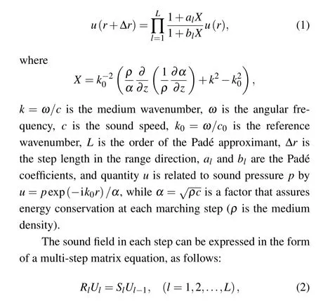
whereLis the order of the Pad′e approximant, matrixUl(l=1,2,...,L) is the discrete form ofuin stepl,RlandSlareN×Nreversible tridiagonal matrices, andNis the depth number of grid points. The chase method can achieve faster calculation speed in actual matrix operation.

From the perspective of mathematical form,the transformation between the same dimensions of column vectors can be realized by multiplying the same dimension square matrix,which can be regarded as the simplest form of vector transformation. Inspired by the aforementioned mathematical ideas,the column vectors obtained by the discrete depth operators at different ranges in the PE model can also be calculated via single equal dimension reversible square matrix multiplication.The square matrix that connects two sound field vectors can be called the propagation matrix.

The recurrence formula for the sound field with the propagation matrix method[31]is expressed as

whereMis the propagation matrix for calculating the sound field at different distances, and it contains the information of the marine environment parameters at the propagation distance. MatrixUis the discrete form ofu.where[φ,φ]represents the inner product of two vectorsφandφ.

Equation (12) is the core formula for mode decomposition theory of the parabolic equation model, which is consistent with NM.The modes of the parabolic equation model can be considered the result of the uniform sampling of NM in the depth direction. The expression of underwater sound pressure can be obtained by the relation between quantityuand sound pressurep,that is,

where Δzis the step length in the depth direction.

Compared with the classic parabolic equation model,propagation decomposition theory of sound field assumes that the different eigenvectors of the propagation matrix satisfy orthogonality and make approximations in two aspects. Firstly,the approximate orthogonal decomposition of the propagation matrix is adopted. When different eigenvectors are orthogonal to one another,no energy exchange occurs among the propagation mode components,which are all independent propagation modes. In fact, the modes are not completely consistent because the propagation matrix cannot be strictly symmetric in ocean sound waveguides. Then,a redistribution of energy occurs when different modes propagate to a long distance, and the role of this phenomenon is disregarded in the new theory. Secondly, the approximate orthogonal decomposition of the initial sound field is adopted. In the process of representing the initial sound field as a linear combination of different eigenvectors,the different eigenvectors are assumed to be orthogonal and the influences of each component on the coefficients are not considered. This approximation disregards the influence of the correlation between modes in the sound field,and it exerts an evident influence on the results of the nearrange sound field. However, the influence on the sound field decreases rapidly with an increase in propagation range.

In accordance with the uniqueness of the sound propagation modes,the new PE mode theory can be used to calculate the wave mode eigenvalues and eigenfunctions. On the basis of normal mode theory,sound pressure can be written as

Then, the PE model establishes a relationship with normal mode theory.

3. Numerical examples

To verify the validity of PM,this section presents a simulation analysis of the sound propagation problem in some representative waveguides, namely, shallow-water, deep-water,and multilayer waveguides.

In next numerical experiment, the normal modes and incoherent transmission loss (TL) lines are calculated by using the NM program KRAKENC[32]and PM.Meanwhile,the coherent TL results are obtained by using PE, NM, and PM. In PM, the setting methods ofL(the order of the Pad′e approximant),Δr(the step length in the range direction),and Δz(the step length in the depth direction)are consistent with those of the RAM-PE method.

3.1. Shallow-water waveguide

In Fig. 1, a 100 Hz source is located atz=50 m, withc1=1500 m/s andρ1=1 g/cm3in the water column. An ocean with a depth of 200 m is overlying a fluid sediment in whichc2=1700 m/s,ρ2=1.5 g/cm3, and attenuation is 0.5 dB/λ. In the experiment,the thickness of the artificial absorption layer is 200 m withL=6,Δr=5,and Δz=1.

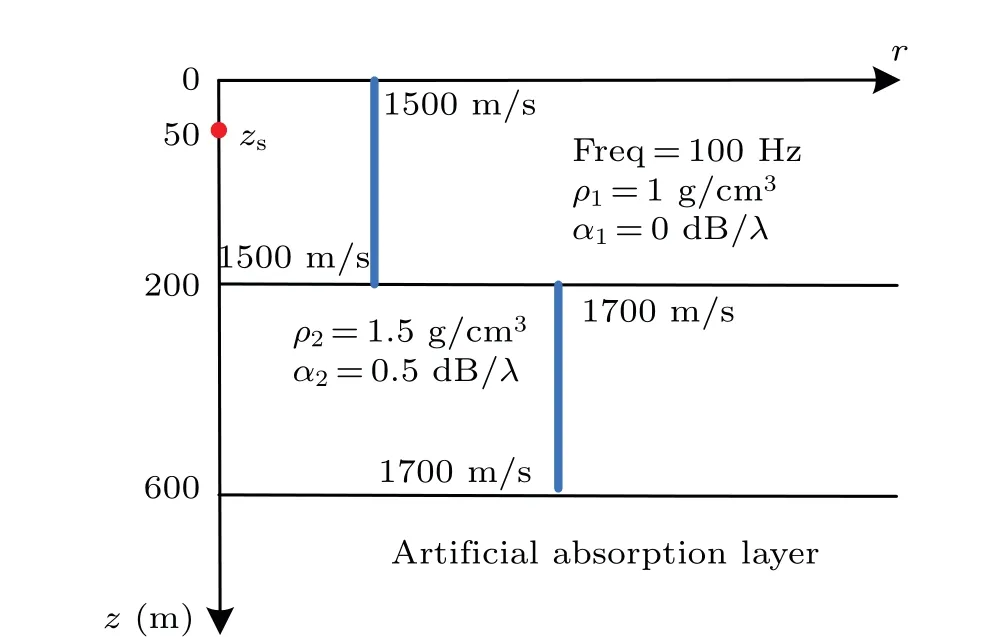
Fig.1. Shallow-water waveguide.

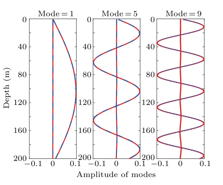
Fig.2. Eigenfunctions in the shallow-water waveguide.

Figure 2 shows the eigenfunctions of modes 1, 5, and 9 calculated by using the NM(the blue dotted line)and PM(the red solid line) solutions. The solid blue line represents the result of NM,while the red dotted line indicates the result of PM.The subsequent experiments are labeled in the same manner. The mode eigenfunction lines are consistent with one another. The normal mode eigenvalue results of NM and PM from modes 1-9 are provided in Table 1. The eigenvalues obtained using PM exhibit good agreement with the results of NM.With an increase in the order of mode,the eigenvalue error between the two methods becomes larger due to the phase error of the PE method. In the experiment,the real and imaginary parts of the eigenvalues of PM are larger than those of NM,indicating that the major PM modes from modes 1-9 exhibit faster phase speed and energy loss. Figure 3 shows the 2D TL results calculated using NM, PM, and RAM-PE. The overall fields are highly similar,and thus,the accuracy of the three methods should be compared further. Figure 4 shows the TL lines calculated using NM,PM,and RAM-PE.The coherent TL lines are highly similar, particularly between PM and RAM-PE. The difference in mode phase speed between NM and PM causes the range expansion of the coherent TL. The PM and RAM-PE TL lines are stretched in the range direction in the shallow-water waveguide. The incoherent TL line of PM is slightly (within 1 dB) smaller than that of NM within 2 km due to the larger imaginary part of mode eigenvalues.This result is in good agreement with NM in the long range.

Table 1. Eigenvalues in the shallow-water waveguide.

Fig.3. TL field in the shallow-water waveguide. (a)NM;(b)PM;(c)RAM-PE.

Fig.4. TL lines in the shallow-water waveguide.

3.2. Deep-sea waveguide

The deep-water waveguide adopts the Munk profile, a typical sound speed profile that can exhibit many features of deep water sound propagation. In the experiment, a 50 Hz source is located atz=50 m. The detailed environment parameters are presented in Fig.5. The thickness of the artificial absorption layer in PE is 1000 m withL=6, Δr=10, and Δz=5.

Fig.5. Deep-water waveguide.

The normal mode eigenvalues and eigenfunctions calculated by using NM and PM are provided in Table 2 and Fig.6,where NM uses the blue dotted line and PM adopts the red solid line.The eigenfunctions of the two methods exhibit minimal difference,including higher-order modes.

Fig.6. Eigenfunctions in the deep-water waveguide.

In contrast with the shallow-water waveguide, the real part of the primary eigenvalues of PM is larger than that of NM, and the phase error of PE leads to a slower propagation speed, as demonstrated by the coherent TL results in Fig. 7.Meanwhile,the order of modes reaches up to several hundreds in the deep-water waveguide,causing a larger TL error in NM and PM.Figure 8 illustrates that the 2D TL results of PM and RAM-PE are consistent with each other and exhibit evident energy difference with NM in the first shadow zone.

Table 2. Eigenvalues in the deep-water waveguide.

Fig.7. TL lines in the deep-water waveguide.

Fig.8. TL field in the deep-water waveguide. (a)NM;(b)PM;(c)RAM-PE.

3.3. Multilayer-bottom waveguide

Compared with the two preceding numerical examples,the multilayer waveguide shown in Fig. 9 is a more complex environment. A 50 m seafloor sediment is set above a semiinfinite seabed with a positive gradient sound speed profile. In the waveguide, a negative gradient sound speed profile is set in the water layer. The depth of the 200 Hz source is 50 m.The density and sound absorption coefficient of the different layers are presented in the figure. The thickness of the artificial absorption layer in PE is 200 m withL=6, Δr=2, and Δz=1.

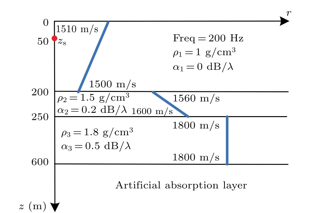
Fig.9. Multilayer-bottom waveguide.

Fig.10. Eigenfunctions in the multilayer-bottom waveguide.

In higher-order modes, the eigenfunction amplitude of PM (the red solid line) is slightly smaller than the result of NM(the blue dotted line),as shown in Fig.10. The eigenvalues calculated using NM and PM also exhibit a complex difference in Table 3. The real part of the PM eigenvalues is larger than that of the NM eigenvalues in higher-order modes. The diverse mode differences between NM and PM cause a more evident error of the TL results calculated using NM and PM than the shallow-water and deep-water waveguides. The influence can be clearly observed in the 2D TL results presented in Fig.11,but it can be demonstrated using the TL lines from Fig.12. In multilayer-bottom waveguides,the validity of NM and PM must be verified in future work.

Table 3. Eigenvalues in the multilayer-bottom waveguide.

Fig.11. TL field in the multilayer-bottom waveguide. (a)NM;(b)PM;(c)RAM-PE.

Fig.12. TL lines in the multilayer-bottom waveguide.

3.4. Discussion

As demonstrated in the previous numerical examples,PE is an effective method for calculating normal mode. The type of sound source in most underwater sound propagation models is omnidirectional,including NM.Through the proposed PM,the normal mode stimulated by certain directional sources can be solved. When the acceptable phase error of PE is set to 0.0002, the angle limitations of Pad′e approximation are approximately 45°[Pad′e(2)] and 90°[Pad′e(8)]. A±45°direction source in the main propagation direction is considered in the following example. To reduce the number of normal modes, two 10 Hz sources are located atz= 1000 m andz= 3000 m in the deep-water waveguide shown in Fig. 5.The thickness of the artificial absorption layer in PE is 1000 m with Δr=20,and Δz=10. The real and imaginary parts of all mode eigenvalues calculated using NM and PM in Pad′e(8)and Pad′e(2)are shown in Figs.13(a)and 13(b). A conclusion can be drawn that the eigenvalues obtained using PM in Pad′e(2)have a considerably larger imaginary part than the results obtained under the two other conditions when the order is above 50. That is, the order of modes above 50 can be disregarded.The grazing angle of mode 50 is approximately 49°,which is consistent with the angle limitation of Pad′e(2). The TL results in Figs.14(a)and 14(b)can also verify the validity of the angle limitations quantitatively.

Fig.13. Mode eigenvalues calculated using NM and PM.(a)Real part;(b)imaginary part.

Fig.14. TL field calculated using PM.(a)Pad′e(8)N=63;(b)Pad′e(2)N=63;(c)Pad′e(8)N=50.

PM can get N modes based on the matrix eigenvalue decomposition method. If the real part of eigenvalues calculated by NM is greater than the real part ofk2(k2=ω/cmax,cmaxis the maximum sound speed on the seabed)and less than the real part ofk1(k1=ω/cmin,cminis minimum sound speed of sea water), it can be called as waveguide normal mode in accordance with NM.

When using NM to calculate the wave mode eigenvalues, it is possible to miss its roots. However, the PM method can solve this problem. Some numerical experiments are carried out by using the shallow-water waveguide in Fig.1. The source frequency is 25 Hz and the depth of sea water adds from 50 m to 200 m with a 5 m interval. Figure 15 shows the number of waveguide normal modes at different seawater depths calculated by using NM and PM.NM has the problem of missing root when the depths of seawater are 120 m,185 m and 200 m,but by using PM can obtain right results. The normal mode eigenvalues at the depth of 120 m,185 m and 200 m are calculated by using NM and PM,which are provided in Table 4. The results prove the advantage of PM.

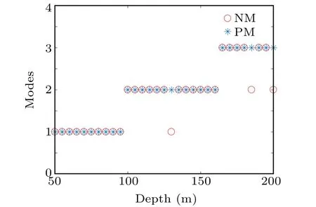
Fig. 15. Number of waveguide normal modes at different seawater depths are calculated by using NM and PM.

Table 4. Eigenvalues at different seawater depths.

4. Conclusion and perspectives

The split-step Pad′e PE model provides a method for calculating wave modes that expands the application of PE models. Numerical experiments on three typical ocean waveguides test the effectiveness and accuracy of PM, although some small errors exist.Compared with the shallow-water and deep-water waveguides,the complex bottom of the multilayerbottom waveguide causes a larger difference between NM and PM. Increased attention is necessary to determine which method is more accurate. Meanwhile, the angle limitation of Pad′e approximation is verified by the results of different orders of Pad′e coefficient in PM and the problem of missing root is also solved by PM.In the future,an elastic PM will be proposed and a smooth wave mode method based on PM will be presented for fluctuating ocean waveguides.

Acknowledgement

Project supported by Young Elite Scientist Sponsorship Program by CAST(Grant No.YESS20200330).